The Synthetic Historical Control Method

Oftentimes, we struggle with picking a donor pool for SCMs due to spillovers or the event being so massive that it is hard to argue for clean donors in principle. This blog post shows you one way we can get around that problem via using the synthetic historical control method. It is a flavor of synthetic controls, as the name suggests.

Notations

The notation for this method (as it is presented in the paper) makes my head hurt, so I will simply quote directly from my paper that currently uses this method in hopes that I can spell it out clearly.

Let \(\mathbb{R}\) denote the set of real numbers, and let \(\|\cdot\|_1\) denote the usual \(\ell_1\) vector norm. Throughout, I denote sets using calligraphic letters (e.g., \(\mathcal{T}, \mathcal{S}, \mathcal{N}\)) for clarity. Scalars are represented using plain lowercase letters (e.g., \(h, t, n, m\)), and matrices are denoted by bold uppercase letters (e.g., \(\mathbf{X}, \mathbf{W}, \mathbf{Y}\)). Given a vector \(\mathbf{x} = (x_1, x_2, \dots, x_T)^\top \in \mathbb{R}^T\) and an index set \(\mathcal{I} \subseteq \{1, \dots, T\}\), I write \(\mathbf{x}_{\mathcal{I}} \coloneqq (x_t)_{t \in \mathcal{I}} \in \mathbb{R}^{|\mathcal{I}|}\) to denote the subvector of \(\mathbf{x}\) corresponding to indices in \(\mathcal{I}\), preserving their original order.

Let \(\mathcal{T} = \{1, 2, \dots, T\}\) index time. Define the pre-treatment period as \(\mathcal{T}_1 \coloneqq \{t \in \mathcal{T} : t \leq T_0\}\) and the post-treatment period as \(\mathcal{T}_2 \coloneqq \{t \in \mathcal{T} : t > T_0\}\). The number of post-treatment periods is \(n = T - T_0\). Let \(m \in \mathbb{N}\) denote the evaluation window length, i.e., the number of periods used to construct the SHC match. Define the evaluation period as the final \(m\) months of the pre-treatment period:

\[ \mathcal{T}_{\text{eval}} \coloneqq \{T_0 - m + 1, \dots, T_0\} \subset \mathcal{T}_1. \]

Let \(\mathbf{y} = (y_1, y_2, \dots, y_T)^\top \in \mathbb{R}^T\) denote the observed outcome vector for the treated unit. Define the pre-treatment outcome vector \(\mathbf{y}_{\text{pre}} \coloneqq \mathbf{y}_{\mathcal{T}_1} \in \mathbb{R}^{T_0}\), the evaluation subvector \(\mathbf{y}_{\text{eval}} \coloneqq \mathbf{y}_{\mathcal{T}_{\text{eval}}} \in \mathbb{R}^m\), and the post-treatment outcome vector \(\mathbf{y}_{\text{post}} \coloneqq \mathbf{y}_{\mathcal{T}_2} \in \mathbb{R}^n\). The evaluation subvector \(\mathbf{y}_{\text{eval}}\) is the target pattern to be reconstructed using convex combinations of earlier segments from the pre-treatment period.

To reconstruct the evaluation window, we compare it against earlier segments of the treated unit’s own pre-treatment trajectory. Define the donor matrix \(\widetilde{\mathbf{Y}}_{\text{pre}} \in \mathbb{R}^{m \times N}\) as a collection of \(N\) overlapping length-\(m\) subvectors extracted from the smoothed pre-treatment series. Each column is a contiguous subvector of the form \(\widetilde{\mathbf{y}}_{[i, i+m-1]}\), with \(i\) ranging over eligible start points in \(\mathcal{T}_1\) that precede the evaluation window.

The Synthetic Historical Control (SHC) Estimator

The SHC method is a synthetic control-style estimator that constructs a counterfactual using only the treated unit’s own historical data. This makes SHC particularly useful when no clean donor units are available, for instance, when all states or countries are exposed to a shock like COVID-19. SHC begins by smoothing the pre-treatment outcome time series \(\{y_t\}_{t=1}^{T_0}\) using local linear regression, which helps reduce noise and better recover the underlying trend. In practice, I use leave one out cross validation to choose the bandwidth for the Gaussain kernel. Either way, the result of all this is a smoothed series:

\[ \widetilde{\mathbf{y}} = (\widetilde{y}_1, \ldots, \widetilde{y}_{T_0})^\top. \]

From this smoothed series, we construct a donor matrix of historical segments by taking overlapping segments of length \(m\):

\[ \widetilde{\mathbf{Y}}_{\text{pre}} = \begin{bmatrix} \widetilde{\mathbf{y}}_{[1, m]} & \widetilde{\mathbf{y}}_{[2, m+1]} & \cdots & \widetilde{\mathbf{y}}_{[N, N+m-1]} \end{bmatrix} \in \mathbb{R}^{m \times N}, \]

where \(N = T_0 - m - n + 1\) and each column is a historical “donor” segment used to predict post-treatment outcomes. In this case, we have \(n\) post-treatment observations.

I do not feel the authors do a good job of this in the paper, so I will give a toy example (and I do this in my current paper, as well, that examines a different case) of how the donor pool is actually built.

Suppose we have \(T_0 = 14\) days of pre-treatment data, and we want to: use \(m = 2\) days to define the evaluation window (i.e., the last 2 days before treatment) and predict \(n = 1\) day into the post-treatment period. Then, to build a valid donor, each segment must be \(m + n = 3\) days long: the first \(m\) days are used to match the evaluation window, and the last \(n\) days are used to forecast the post-treatment period.

So, how many such segments can we extract from the 14 pre-treatment days? We need to ensure that each 3-day segment fits entirely within the pre-treatment window. The last such segment would be \((\widetilde{y}_{12}, \widetilde{y}_{13}, \widetilde{y}_{14})^\top\). Thus, the total number of eligible segments is: \[ N = T_0 - m - n + 1 = 14 - 2 - 1 + 1 = 12. \]

Each donor segment looks like: \[ \widetilde{\mathbf{y}}_{[i, i + m + n - 1]} = (\widetilde{y}_i, \widetilde{y}_{i+1}, \widetilde{y}_{i+2})^\top \quad \text{for } i = 1, \dots, 12. \]

The first \(m = 2\) elements are used for fitting the evaluation window. The final \(n = 1\) element is used to extrapolate into the post-treatment period. So the donor matrix for evaluation looks like: \[ \widetilde{\mathbf{Y}}_{\text{pre}} = \begin{bmatrix} \widetilde{y}_1 & \widetilde{y}_2 & \cdots & \widetilde{y}_{12} \\ \widetilde{y}_2 & \widetilde{y}_3 & \cdots & \widetilde{y}_{13} \end{bmatrix} \in \mathbb{R}^{2 \times 12}, \] and the corresponding donor matrix for forecasting (aligned with each segment’s next day) is: \[ \widetilde{\mathbf{Y}}_{\text{post}} = \begin{bmatrix} \widetilde{y}_3 & \widetilde{y}_4 & \cdots & \widetilde{y}_{14} \end{bmatrix} \in \mathbb{R}^{1 \times 12}. \]

We use the pre period for the historical controls to fit our evaluation period for our treated unit. As in normal SCM style, all of those weights are applied to the full segment matrix to give us the in and out of sample predictions. So the SHC counterfactual for day 15 is estimated as: \[ \widehat{y}_{15} = \widetilde{\mathbf{Y}}_{\text{post}} \cdot \mathbf{w}^\ast, \] where \(\mathbf{w}^\ast\) are weights that optimally match the evaluation window using the \(\widetilde{\mathbf{Y}}_{\text{pre}}\) matrix.

SHC selects weights \(\mathbf{w} \in \mathbb{R}^N\) to minimize the squared distance between the evaluation window and a convex combination of donor segments. We also have a penalty term:

\[ \mathbf{w}^\ast = \arg\min_{\mathbf{w} \geq 0, \ \mathbf{1}^\top \mathbf{w} = 1} \left\| \widetilde{\mathbf{y}}_{\text{eval}} - \widetilde{\mathbf{Y}}_{\text{pre}} \mathbf{w} \right\|_2^2 + \varsigma \left\| \mathbf{C}_0^\top \mathbf{w} \right\|_2^2. \]

The term on the left is the ususal OLS loss function. Here, \(\mathbf{C}_0\) contains the eigenvectors of the donor pool’s Grammian matrix. We use this term to stabilize the optimization, since in practice we will always have more predictors than the segment length allows. The authors go into more detail on this in their paper on page 11.

Choosing Our Historical Segments

To avoid using too many donor segments and overfit, SHC implements a forward selection algorithm. The authors in the paper sort of choose an arbitrary number of donors to use. They find that 27 donor segments about does the job, in practice. However, I did not like that they wanted to use a stepwise method with no stopping rule, since this just means that the size of the donor pool we use is kind of arbitrary. So, I write my own forward selection method. Starting with an empty set, it adds one donor at a time, each time choosing the segment that most reduces the in-sample MSE.

\[ \mathcal{S}_j = \mathcal{S}_{j-1} \cup \left\{ \underset{i \in \mathcal{N} \setminus \mathcal{S}_{j-1}}{\operatorname*{argmin}} \left\| \widetilde{\mathbf{y}}_{\text{eval}} - \widetilde{\mathbf{Y}}_{\text{pre}}^{(\mathcal{S}_{j-1} \cup \{i\})} \mathbf{w}^{(j)} \right\|_2^2 + \varsigma \left\| \mathbf{C}_0^\top \mathbf{w} \right\|_2^2 \right\}, \quad \mathcal{S}_0 = \emptyset, \]

To choose when to stop adding donors, we compute a modified BIC at each step:

\[ \text{BIC}(j) = m \cdot \log\left( \text{MSE}_j \right) + \lambda j, \]

where \(\text{MSE}_j\) is the in-sample mean squared error using \(j\) donors, and \(\lambda = \log(m)\). The algorithm stops when BIC increases for two steps in a row. Presumably, we could use a better one, so if you have suggestions let me know. I borrowed this idea from the forward selected PDA approach.

Estimation in Python

In order to get these results, you need Python (3.9 or greater) and mlsynth, which you may install from the Github repo. You’ll need the most recent version.

pip install -U git+https://github.com/jgreathouse9/mlsynth.git

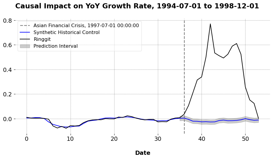
This example uses the Malaysian Ringgit as an example. Its currency was affected by the Asian Financial Crisis. I use the SHC method to estimate the impact the crisis had on the growth rate of the spot exchange rate, taken from FRED’s database. We can see my code below, where I use 36 months (3 years) of a pretreatment period.

from mlsynth import SHC
import pandas as pd


url = "https://fred.stlouisfed.org/graph/fredgraph.csv?bgcolor=%23ebf3fb&chart_type=line&drp=0&fo=open%20sans&graph_bgcolor=%23ffffff&height=450&mode=fred&recession_bars=on&txtcolor=%23444444&ts=12&tts=12&width=1320&nt=0&thu=0&trc=0&show_legend=yes&show_axis_titles=yes&show_tooltip=yes&id=EXMAUS&scale=left&cosd=1971-01-01&coed=2025-06-01&line_color=%230073e6&link_values=false&line_style=solid&mark_type=none&mw=3&lw=3&ost=-99999&oet=99999&mma=0&fml=a&fq=Monthly&fam=avg&fgst=lin&fgsnd=2020-02-01&line_index=1&transformation=lin&vintage_date=2025-07-17&revision_date=2025-07-17&nd=1971-01-01"

df = pd.read_csv(url)

df.rename(columns={df.columns[0]: "Date"}, inplace=True)
df["Date"] = pd.to_datetime(df["Date"])

value_col = df.columns[1]
df["YoY Growth Rate"] = df[value_col].pct_change(periods=12)

df = df.dropna(subset=["YoY Growth Rate"])

df = df.drop(columns=df.columns[1])
df = df[df["Date"].dt.year < 1999]

df["Unit"] = "Ringgit"

df["Asian Financial Crisis"] = (df["Date"] >= pd.Timestamp("1997-07-01")).astype(int)

config = {
    "df": df,
    "outcome": df.columns[1],
    "treat": df.columns[-1],
    "unitid": "Unit",
    "time": df.columns[0],
    "display_graphs": True,
    "save": False,
    "counterfactual_color": ["blue"], "m": 12*3
}

result = SHC(config).fit()

MSE with best 1 donors: 0.0009644526 | BIC: -246.398676
MSE with best 2 donors: 0.0002455641 | BIC: -292.063246
MSE with best 3 donors: 0.0001905261 | BIC: -297.615414
MSE with best 4 donors: 0.0001623415 | BIC: -299.795017
MSE with best 5 donors: 0.0001421587 | BIC: -300.990811
MSE with best 6 donors: 0.0001020778 | BIC: -309.330798
MSE with best 7 donors: 0.0000876191 | BIC: -311.245787
MSE with best 8 donors: 0.0000734166 | BIC: -314.028821
MSE with best 9 donors: 0.0000644736 | BIC: -315.121485
MSE with best 10 donors: 0.0000599316 | BIC: -314.167843
MSE with best 11 donors: 0.0000551007 | BIC: -313.609795
Stopping early at j=11 due to BIC increase.

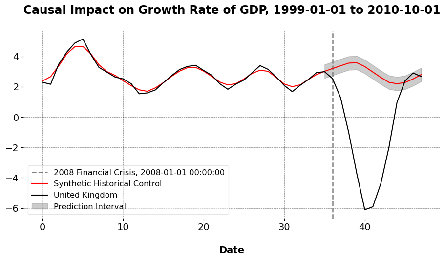
Now I do the effect of the 2008 Financial Crisis, because why not? I look at the effet for the U.K., but of course we may choose any nation we like. I use the precomputed annual growth rate of GDP.

url ="https://fred.stlouisfed.org/graph/fredgraph.csv?bgcolor=%23ebf3fb&chart_type=line&drp=0&fo=open%20sans&graph_bgcolor=%23ffffff&height=450&mode=fred&recession_bars=off&txtcolor=%23444444&ts=12&tts=12&width=1320&nt=0&thu=0&trc=0&show_legend=yes&show_axis_titles=yes&show_tooltip=yes&id=GBRGDPRQPSMEI&scale=left&cosd=1956-01-01&coed=2025-01-01&line_color=%230073e6&link_values=false&line_style=solid&mark_type=none&mw=3&lw=3&ost=-99999&oet=99999&mma=0&fml=a&fq=Quarterly&fam=avg&fgst=lin&fgsnd=2020-02-01&line_index=1&transformation=lin&vintage_date=2025-07-17&revision_date=2025-07-17&nd=1956-01-01"

df = pd.read_csv(url)

df.rename(columns={df.columns[0]: "Date", df.columns[1]: "Growth Rate of GDP"}, inplace=True)
df["Date"] = pd.to_datetime(df["Date"])
value_col = df.columns[1]

df = df[df["Date"].dt.year < 2011]
df["Unit"] = "United Kingdom"
df["2008 Financial Crisis"] = (df["Date"] >= pd.Timestamp("2008-01-01")).astype(int)

configFC = {
    "df": df,
    "outcome": df.columns[1],
    "treat": df.columns[-1],
    "unitid": "Unit",
    "time": df.columns[0],
    "display_graphs": True,
    "save": False,
    "counterfactual_color": ["red"], "m": 36
}

resultFC = SHC(configFC).fit()

MSE with best 1 donors: 0.8375617331 | BIC: -2.797852
MSE with best 2 donors: 0.2285861877 | BIC: -45.963272
MSE with best 3 donors: 0.1793404556 | BIC: -51.114338
MSE with best 4 donors: 0.1016206983 | BIC: -67.980214
MSE with best 5 donors: 0.0404368881 | BIC: -97.570867
MSE with best 6 donors: 0.0191391750 | BIC: -120.915534
MSE with best 7 donors: 0.0124970903 | BIC: -132.676707
MSE with best 8 donors: 0.0100946176 | BIC: -136.778953
MSE with best 9 donors: 0.0086642921 | BIC: -138.695952
MSE with best 10 donors: 0.0072633615 | BIC: -141.461662
MSE with best 11 donors: 0.0056592847 | BIC: -146.861772
MSE with best 12 donors: 0.0053809976 | BIC: -145.093507
MSE with best 13 donors: 0.0047071484 | BIC: -146.326482
MSE with best 14 donors: 0.0028529738 | BIC: -160.768897
MSE with best 15 donors: 0.0024030221 | BIC: -163.364229
MSE with best 16 donors: 0.0010180807 | BIC: -190.697797
MSE with best 17 donors: 0.0008640748 | BIC: -193.018824
MSE with best 18 donors: 0.0005711405 | BIC: -204.340169
MSE with best 19 donors: 0.0004850733 | BIC: -206.636720
MSE with best 20 donors: 0.0004385279 | BIC: -206.684756
MSE with best 21 donors: 0.0003952938 | BIC: -206.837832
MSE with best 22 donors: 0.0003804762 | BIC: -204.629716
MSE with best 23 donors: 0.0003661885 | BIC: -202.424107
Stopping early at j=23 due to BIC increase.

The ATT for the growth rate is -3.755, meaning the economy shrank by 3 percentage points over the next three years following the 2008 Financial Crisis/Crash.

Of course, these examples are both financial crises, but you can literally do this with anything that we have a big enough time series to do it with. No reason this method cannot work with promotions for sales of goods, ad campaigns, tourism (my current applicattion!) or other questions we may care about.

Caveats

The authors note that this approach will not work with trendy data (which makes sense due to the convex combination of donor periods). In other words, you need to detrend it first if a trend exists. This is why I use the growth rate to (ideally) avoid this issue.

In principle, I like this method. I wonder what would happen if we just did this same method of donor pool construction, but just slapped on the Robust SCM method for the weight solution, where we take the low rank structure of the pre-treatment period and learn the weights via OLS. Unclear as to whether/why we could not do this, or add in other penalty type terms or intercepts to adjust for this, either.. If the idea is just that “we think the future will look like some combination of the untreated past”, then who’s to say that using the low-dimensional subspace of pre-treatment periods wouldn’t be a good idea? The authors do not propose inference methods either, so I use the agnostic conformal prediction intervals from the scpi package. Presumably though there’s a better way than this.

Anyways, all of that is really for another paper. The SHC method itself is not even published just yet, so unclear how popular it will become or if others will want to extend it for other things. But now of course, you too may use it, should you wish.