The Synthetic Control Method
2025-11-11
Applied Averages
In real life, weights are never handed down from the heavens: we, the econometricians, must assign them. Assigning them poorly can produce nonsensical averages if we wish to use averages as comparisons, as we often do.
The arithmetic average is familiar to applied economists, coming up sometimes as the national average. It is used all the time in policy discussions, for example:
But again, this assumes that the aggregate weights produce a meaningful comparison for a single unit — which may not be true (recall the Bill Gates example).
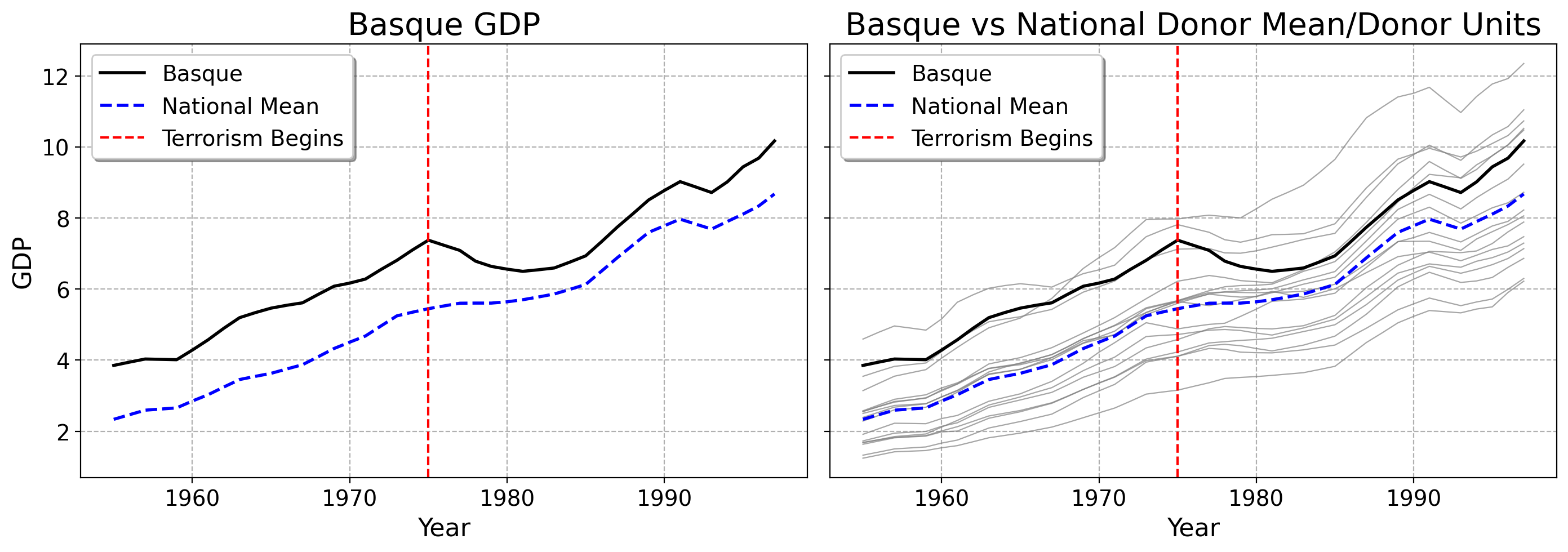
Suppose we have one unit exposed to terrorism in 1975 (the Basque Country), and a set of 16 other units that are not exposed. We want to estimate the effect of terrorism on GDP per capita. How to choose the weights?
The Basque Country is much wealthier than many areas of Spain, has a unique political climate, and was more educated and industrialized than other areas.
Optimization can solve this problem. Instead of us just arbitrarily assigning weights, we choose the weights that minimize the pre-intervention gap between the Basque Country and the weighted donor units.
Least Squares Cont.
Here are the weights OLS returns to us for the 16 donor units:
| regionname | Weight |
|---|---|
| Andalucia | 4.17551 |
| Aragon | -1.50358 |
| Baleares (Islas) | -0.0107201 |
| Canarias | -0.0168126 |
| Cantabria | 0.261694 |
| Castilla Y Leon | 6.07601 |
| Castilla-La Mancha | -2.6561 |
| Cataluna | -0.945626 |
| Comunidad Valenciana | 0.860017 |
| Extremadura | -1.93895 |
| Galicia | -2.96441 |
| Madrid (Comunidad De) | 0.343366 |
| Murcia (Region de) | -0.620705 |
| Navarra (Comunidad Foral De) | 0.583705 |
| Principado De Asturias | 0.51578 |
| Rioja (La) | -0.94721 |
Notice that OLS assigns some positive and some negative weights. These tell us how similar the control units is to the treated unit. Notice how some units have negative weights. These can be hard to interpret substantively: which units are truly most similar to the Basque Country before terrorism happened? Is it Andalucia or Castilla Y Leon?
Here are some of the predicted donors plotted against the Basque Country
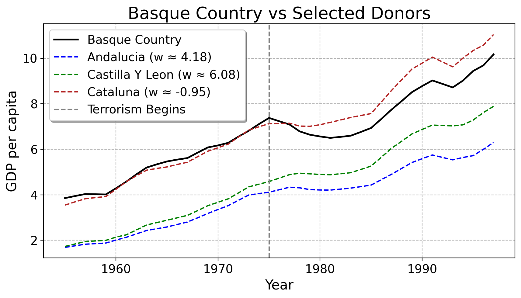
Much of this does not really square very nicely with intution. Cataluna, which is very close to the Basque Country (both literally in terms of GDP and being a French border region in Northern Spain) gets negative weight from OLS. The units which are much farther away from the Basque Country (on top of having much different political/economic histories) get much more weight
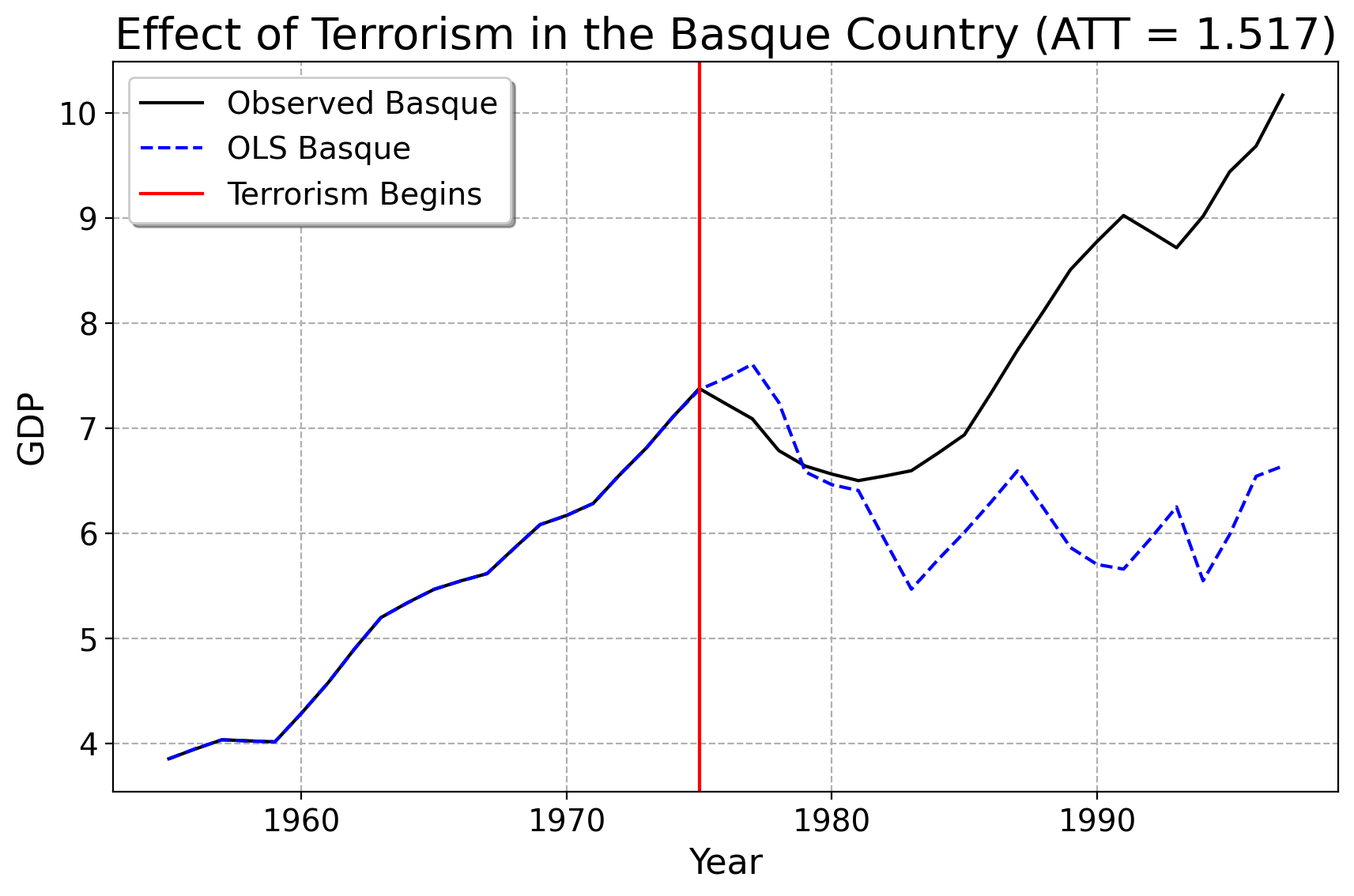
Here is our prediction using OLS. Unfortunately, while OLS fits very well to the Basque Country before terrorism happened, the out-of-sample/post-1975 predicions exhibits a lot more variance than any control unit in the pre-treatment period did. The counterfactual has a weird zig-zag-y prediction. We can see that the prediction line for the Basque country suggests that its economy would have fallen off a cliff, had terrorism not happened. In other words, if the OLS estmate is to be taken seriously, the onset of terrorism saved the Basque economy… This does not seem like a sensible finding historically, or a very reasonable prediction statistically.
How To Change The Weights
What if we could adjust the weights so the synthetic Basque stays within the range of the donor units?
In other words, we want the model predictions to lie inside the full range of the donors only.
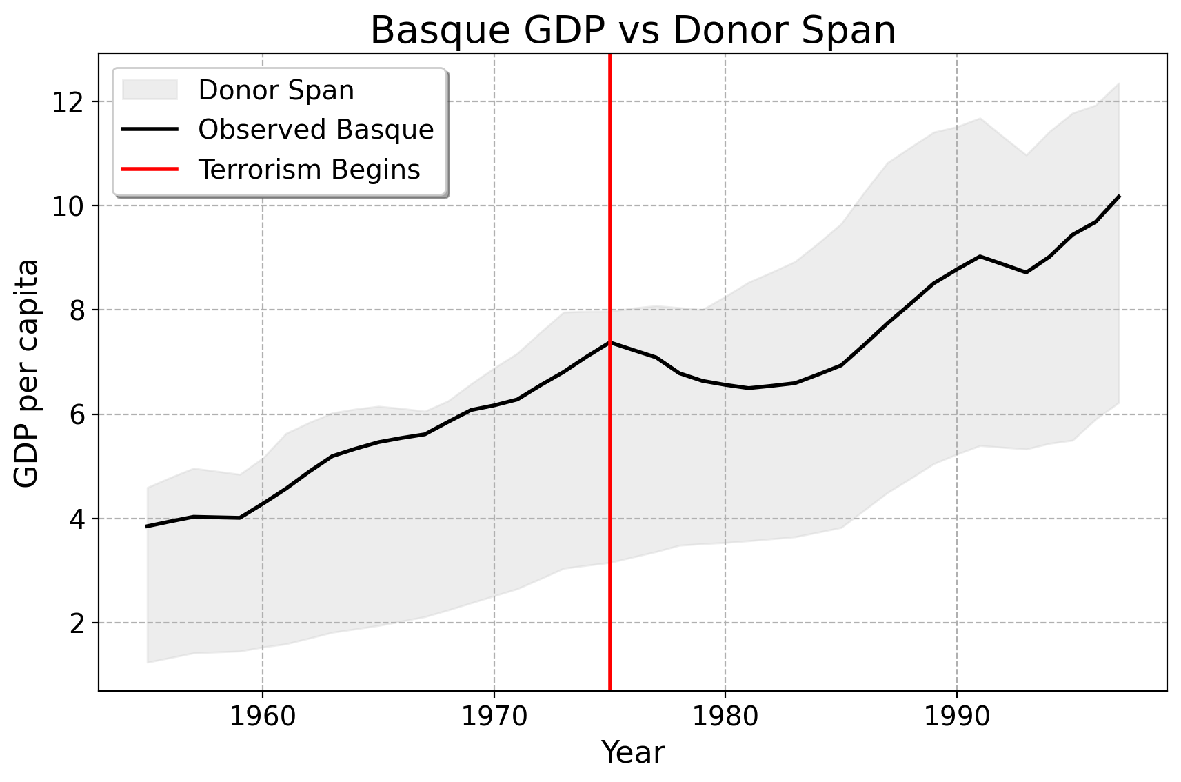
The plot below shows the area spanned by all donor regions in Spain (shaded), along with the Basque Country. This visualizes the full feasible range for any weighted average of donors.
SCM for Basque
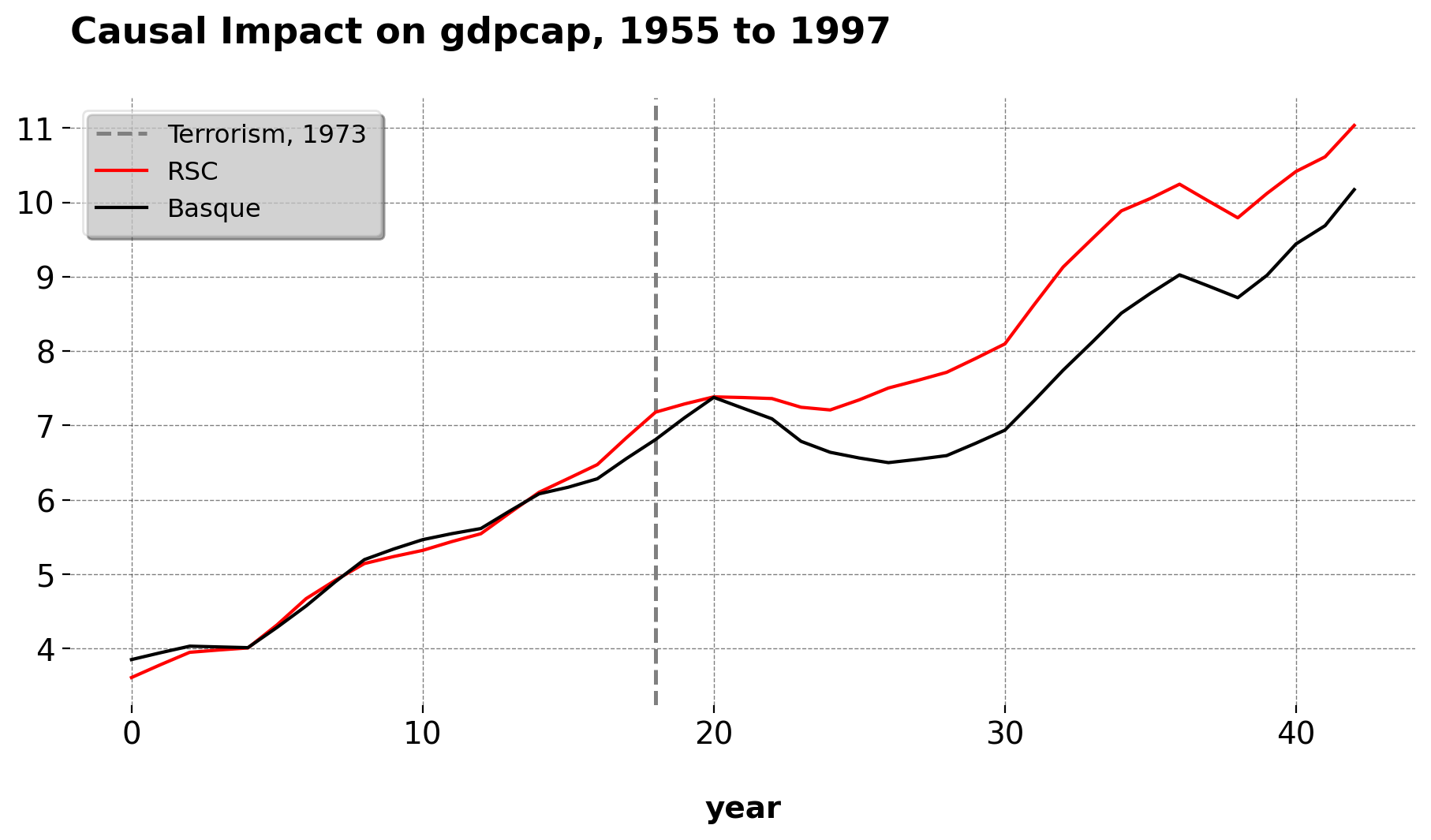
- Here is the result of the regression model. The Basque Country is best reproduced by 85% Catalonia and 15% Madrid.
Convex Combination
Inference: Placebos
Validating SCM designs are important as well, Consider a few robustness checks:
ideally, shifting the treatement back in time should not change the practical results of the conclusions very much.
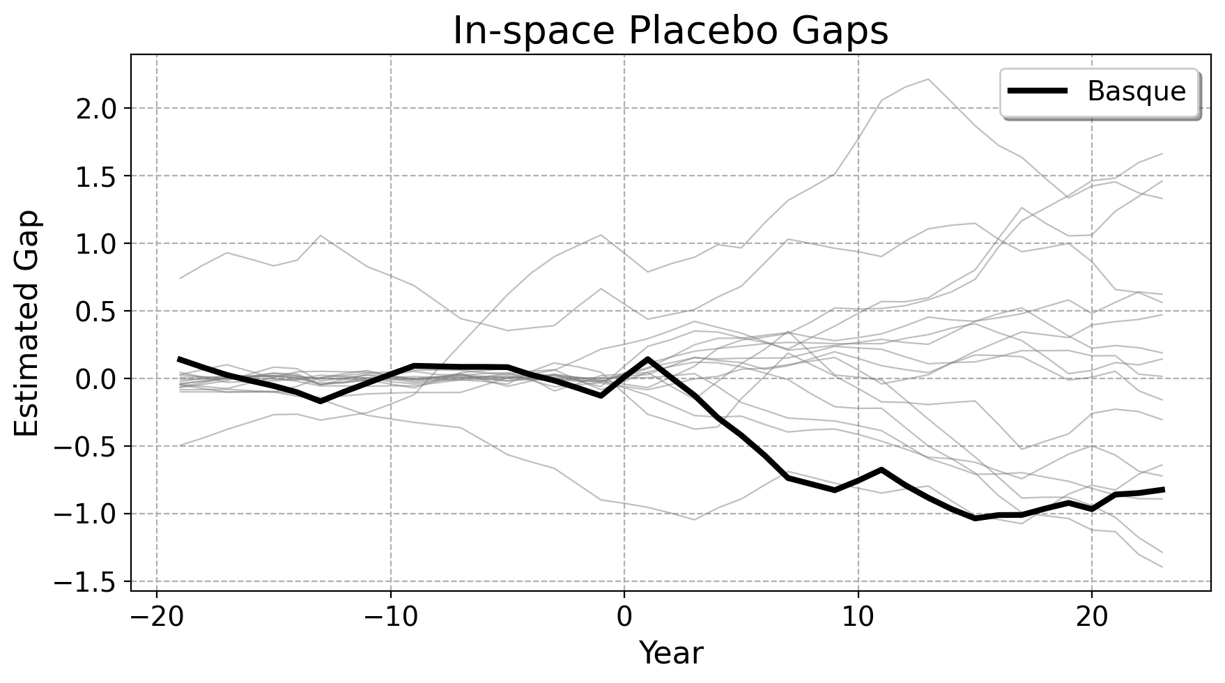
ideally, the treated unit’s treatment effect should look extreme compared to the placebo effect given to other untreated units. Here, we rerun the SCM over the other donor units.
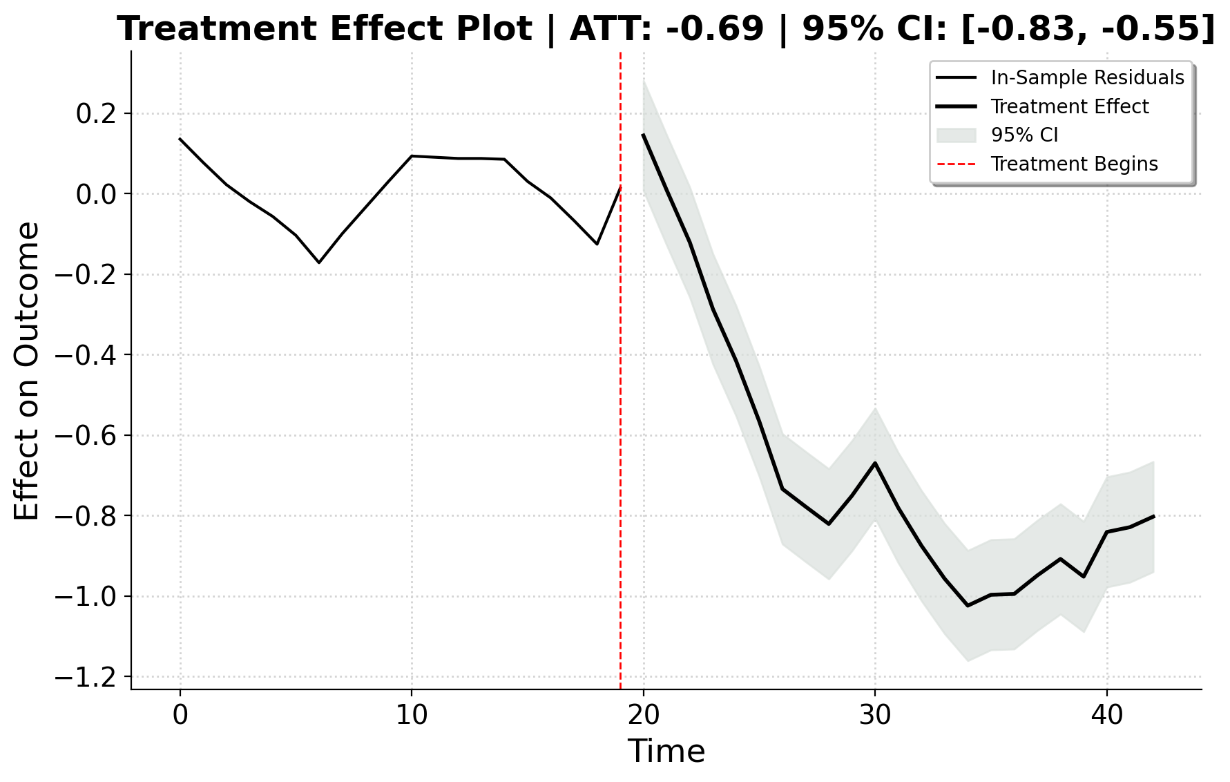
Block Results
Here are our results.
Extensions
Synthetic Control methods have undergone many advances since their inception. If you wish to use Python to estimate synthetic controls, I wrote the largest such package that exists. See here for details: