Causal Inference Runs the World: Actionable Insights, Econometrics Style

What Even Are Actionable Insights, Anyways?

Man, I hate industry jargon. Don’t get me wrong, I’m not against all jargon. I’ve been in academia ten years, and I’ve spent maybe 6 of those being tormented by econometrics. We have our own jargon too, which doesn’t always jive very well with industry- I say “causal inference”, marketers will say “incrementality testing”. I say “experiment”, others say “A/B testing”. I say “practical significance”, others say “value”. There’s something about the data science industry lingo that irritates me. “Ambiguity” (I’ll do a post on this one, one day). “Self starter”. “Business acumen”. And the favorite of the day, “actionable insights.” This post is dedicated to showing you how I think about actionable insights. I approach this from the perspective of somebody who cares a lot about causal inference. I would like to focus on how we can use causal methods from econometrics to deliver actionable insights… But I’m getting ahead of myself.

“Actionable insights”. It’s what we hear about all the time, even if it isn’t phrased exactly like that. Job descriptions and data science pages will go on and on about how we’re meant to deliver them as econometricians, policy analysts, and data scientists. Our livelihoods are essentially staked to producing them. But, what are actionable insights anyways? Some pages say ““Actionable insights” describes contextualised data analysis. It’s a piece of information that can actually be put into action — supported by the analysis, context and communication tools required to get the job done.” I agree with this. This leads us to one question then: how do we know which insights are actionable? And, more pressingly, how do we prodcue these in the first place?

A Motivating Example

Recently I saw a post on LinkedIn. It went something like this:

Data Science Intern: “This is a chart of our App download trends.” Client: “So?”

Junior Data Scientist: “The chart shows that downloading of the App increased by 45%, compared to the same time yesteryear.” Client: “Great! Why?”

Principal Data Scientist: “The chart shows that downloading of the App increased by 45%, compared to the same time yesteryear due to our new pricing strategy. We should roll out Pricing Strategy in more markets since it’ll likely increase revenue by Big Amount.” Client: “That’s great! We’ll get right to it.”

In context, the post was about connecting your results to the next steps of actions businesses/clients should take, saying that context is key to making business recommendations. And that’s great, we should all be doing that. But I find the hypothetical Principal DS’s answer to be quite wanting. I do not understand why we are meant to see the Principal DS’s remarks as any more wise than the Junior DS. Why?

The Principal DS was implicitly making a counterfactual claim in this example. They were explaining to the client that their Policy W had X impact on Outcome Y, an even went as far as to say that if we kept doing Policy W, we may see gains elsewhere in the future. And this may be true. But how can we tell? For all the talk we have about showing impact (instead of telling what you did descriptively), surely we can do better than this. How? Causal inference.

Here is my issue with the post: the second you add the phrase “Impact X happened given our new pricing strategy/policy/other intervention”, we’re now very far aflung from Descriptiville, stuck in Counterfactual Land. In this domain, the laws work differently. You will never get by if the most you can do is simply getting Tableau/BI to make us a chart. Here you see, we need to have some estimate of how sales (or whatever metric we’re meant to care about) would’ve evolved ABSENT whatever the new policy was. Put differently, you can’t just show a bar chart and say “You should do X cuz I made this chart and have verbally attached an explanation to why we see a number”. It requires A LOT more work than that.

Actionable Insights, Econometrics Style

Here is how I think about answering questions in the business context, especially in the setting of marketing/policy analysis.

Defining the Problem

Suppose we work for Uber. Uber introduced Uber Green in September of 2020, as an initiative that is meant to (among other things) incentivize drivers to use electric cars/low emissions vehicles. Suppose our supervisor tasks us with evaluating whether this policy in fact affected the number of drivers who use electric cars, as was the intended goal. Given this situation, we must roll out this intervention someplace first in order to see how it may work in other markets (say, Sayulita, Mexico), and we must generate a counterfactual. Or, the number of drivers who would have used electric cars but for Uber Green’s introduction. In order to accomplish this task, I will use synthetic control based methodologies to estimate the impact. Of course, the goal here is to compute the average treatment effect on the treated, or the average of the differences between our treated unit and the out-of-sample predictions (post intervention period). This allows us to have a summary statistic of the causal effect, as an averge or as a total.

Solving the Problem

Let \(\mathcal{N}\) denote the set of cities indexed by \(j\), where \(N \coloneqq |\mathcal{N}|\) represents the total number of markets. Sayulita, the treated city, is indexed by \(j = 1\), while the set of control cities is denoted by \(\mathcal{N}_0 \coloneqq \mathcal{N} \setminus \{1\}\), with cardinality \(N_0 \coloneqq |\mathcal{N}_0|\). Time periods are indexed by \(t\), with pre-intervention periods \(\mathcal{T}_1 \coloneqq \{1, 2, \dots, T_0\}\) and post-intervention periods \(\mathcal{T}_2 \coloneqq \{T_0+1, \dots, T\}\), where \(T_0\) is the last period before the intervention.

For each market \(j\), let \(\mathbf{y}_j \coloneqq [y_{jt}, \dots, y_{jT}]^\top \in \mathbb{R}^{T}\) represent the vector of new drivers who use electric cars, where \(y_{jt}\) denotes the number of weekly new drivers in market \(j\) at time \(t\). Let \(\mathbf{Y}_0 \coloneqq (\mathbf{y}_j)_{j \in \mathcal{N}_0} \in \mathbb{R}^{T \times N_0}\) be the matrix of control markets that did not do this intervention at this time. To estimate the counterfactual new driver supply in Sayulita, we construct a synthetic control by taking some weighted average of the control markets based on their pre-intervention trends, \(\hat{\mathbf{y}}_1(0) = \mathbf{Y}_0 \mathbf{w}^\top\), where \(\mathbf{w} \in \mathbb{R}^{N_0}\) is a vector of weights assigned to the control cities. These weights are chosen to minimize some loss function. The treatment effect at time \(t\) is then estimated as the difference between the observed and counterfactual outcomes, \(\widehat{\Delta}_t \coloneqq y_{1t} - \hat{y}_{1t}(0)\). Our result of interest is the average of these treatment effects over the post-intervention period:

\[ \widehat{ATT} \coloneqq \mathbb{E}_2[\widehat{\Delta}_t] = \frac{1}{T_2} \sum_{t \in \mathcal{T}_2} \widehat{\Delta}_t. \]

If the introduction of Uber Green in Sayulita leads to an increase in the number of new drivers who use electric vehicles, we expect \(\widehat{\Delta}_t\), we can then comment on how this program may be applied to other areas.[^1]. The observed new drivers who use electric cars in Sayulita follows a factor model:

\[ \mathbf{y}_1 = \mathbf{\Gamma} \mathbf{F} + \boldsymbol{\nu}_1 + \boldsymbol{\delta} \mathbb{1}(t \geq T_0), \]

where \(\mathbf{\Gamma} \in \mathbb{R}^{1 \times k}\) represents the factor loadings, \(\mathbf{F} \in \mathbb{R}^{k \times T}\) is the matrix of latent common factors, and the factors evolve as:

\[ \mathbf{F}_t = \rho \mathbf{F}_{t-1} + \boldsymbol{\eta}_t, \quad \boldsymbol{\eta}_t \sim \mathcal{N}(\mathbf{0}, \mathbf{I}_k), \]

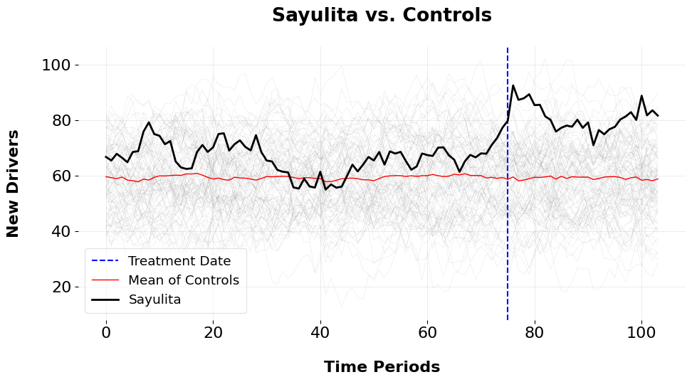
where \(\rho\) is the autocorrelation parameter and \(\boldsymbol{\eta}_t\) is a noise term. The idiosyncratic error term, \(\boldsymbol{\nu}_1\), is assumed to follow a normal distribution with zero mean and variance \(\sigma^2\), i.e., \(\boldsymbol{\nu}_1 \sim \mathcal{N}(\mathbf{0}, \sigma^2 \mathbf{I})\). The treatment effect vector \(\boldsymbol{\delta} \coloneqq [\delta_{T_0+1}, \dots, \delta_T]^\top\) represents the change in driver supply due to the Uber Green intervention, which is assumed to affect Sayulita starting at time \(T_0+1\).

Let’s begin by plotting our outcome. The plot depicts the weekly new Uber drivers who have switched to electric vehicles. Sayulita is our target unit in black, the average of the control group is the thin red line, and the thin grey line are our donors that didn’t enact the intervention.

A few things are apparent: for one, the parallel trends assumption doesn’t apply here across the 75 pre-treatment periods. The mean of controls doesn’t mirror the trend of Sayulita. So, we must use something a little more sophisticated than the standard Difference-in-Differences method. Furthermore, these donors have pretty noisy outcome series. Fortunately, we can exploit the low rank structure of our control group and use that to learn the weights which reconstructs the pre-intervention time series for our treated unit. I’ve written more about this here. Basically, we denoise the data via PCA or functional analysis, and cluster over the functional representation of control units or their right singular values, and extract the donor pool from this low-rank representation. We can then use principal component regression or robust principal component regression to learn our unit weights.

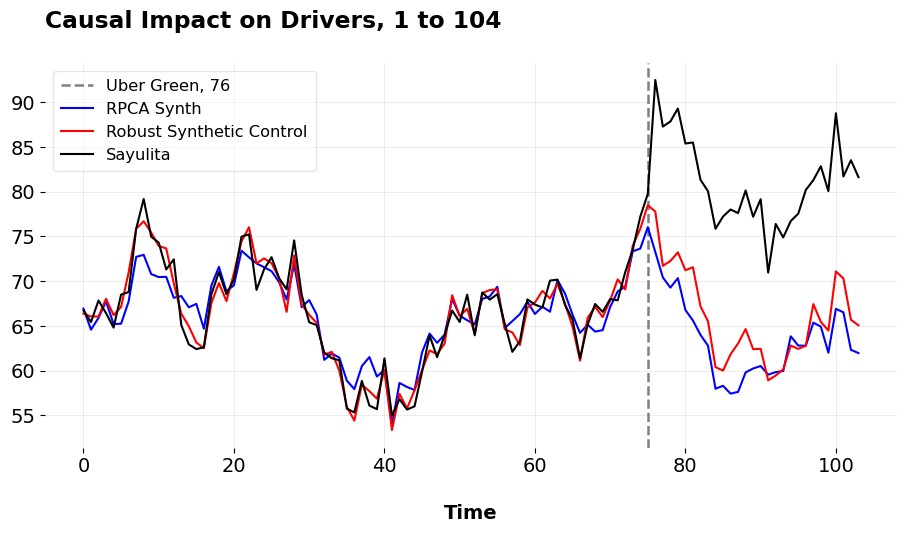
When we do this, we obtain these predictions, of course using my mlsynth to fit the pre-intervention period.

	Metric	RSC	RPCASC
0	Pre-Treatment RMSE	1.263	2.285
1	ATT	14.875	17.312
2	Percent ATT	22.473	27.154

We can see that both the Robust PCA Synthetic Control and the Robust Synthetic Control/Principal Component Regression methods fit Sayulita quite well in the pre-intervention period. They also have very similar ATTs, suggesting that Uber Green increased new electric vehicle use amongst its drivers by anywhere from 22.473 to 26.425 percent. The normal ATTs are also pretty close to the what I simulated, an ATT of 15. Next, I’ll simulate the ATT using Forward Difference-in-Differences.

	Metric	FDID	DID
0	ATT	15.527	14.957
1	Pre-Treatment RMSE	2.315	5.572
2	Percent ATT	23.691	22.624

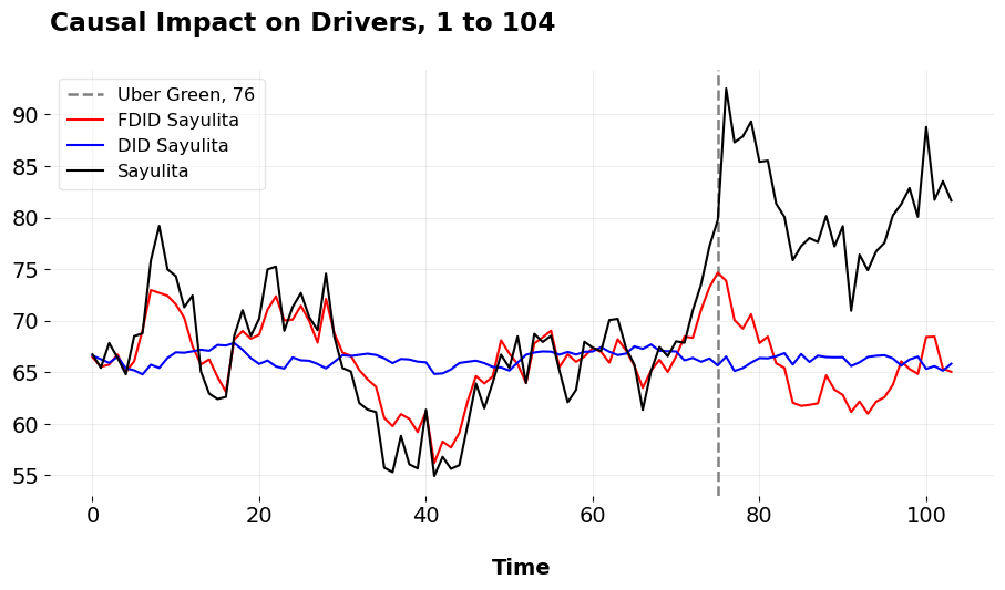
Here we plot the results of the standard Difference-in-Differences design and the Forward DID method. As we can see, parallel pre-intervention trends doesn’t hold at all. The selected parallel trends made by FDID is a lot more sensible in this instance, fitting as well as the synthetic control methods as above.

Just to go really crazy, I decided to combine my estimates into a convex average. Let \(K\) denote the number of counterfactual models, in our case 3. Define \(\mathbf{A} \in \mathbb{R}^{T \times K}\) as the matrix of counterfactual vectors, where each column corresponds to a model and each row represents a time period. The optimization problem is formulated as:

\[ \min_{\mathbf{w} \in \Delta_K} \left\| \mathbf{y}_1 - \mathbf{A} \mathbf{w} \right\|_2 \]

where \(\mathbf{w}\) belongs to the simplex:

\[ \mathbf{w} \in \Delta_K = \left\{ \mathbf{w} \in \mathbb{R}_{\geq 0}^K \mid \left\| \mathbf{w} \right\|_1 = 1 \right\}, \]

or the set spanned by the convex hull of the differing model predictions.

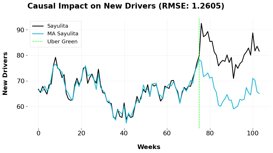
The ATT we compute is 14.902. Just as a very technical note, we see that the RMSE here with the model averaged estimator is lower than any other model I’ve estimated so far. This is because of Jensen’s inequality. Jensen’s inequality states that for a convex function \(f\) and a set of inputs, the function’s value at the weighted average is less than or equal to the weighted average of the function’s inputs:

\[ f\left(\sum_{k=1}^{K} w_k A_k\right) \leq \sum_{k=1}^{K} w_k f(A_k). \]

In our case, we consider the function of the MSE. Due to the quadratic term, \(f(x) = x^2\), we have a convex function. Applying Jensen’s inequality to our loss function, we have

\[ \text{MSE}(\mathbf{w}^\top \mathbf{A}) = \mathbb{E} \left[ (\mathbf{y}_1 - \mathbf{w}^\top \mathbf{A})^2 \right] \leq \sum_{k=1}^{K} w_k \mathbb{E} \left[ (\mathbf{y}_1 - A_k)^2 \right], \]

which essentially guarantees that our model averaged pre-treatment MSE must be lower than the MSE of one of these models by themselves.

Communicating Actionable Insights

Why is this approach superior than simply showing a chart/bar graph? With these results, we can communicate findings easier than before. Instead of simply speculating, we can say, for example,

We simulated the effect of Uber Green four times. Our best estimates suggest that the percentage of new drivers who use electric cars increased between 22.473 and 26.4 percent in the weeks following the Uber Green program being introduced (I also here might use the Bayesian prediction intervals from RSC to comment on uncertainty). When we combined our best three models together, Uber Green added 15 more electric car drivers on average per week. The program added around 488 more electric car drivers than what we would’ve seen otherwise. We would need to roll out the program in new areas for more confirmation, but the evidence suggests Uber Green increases electric car usage.

See how I’m not simply speculating with a bar chart? The value added here is that I’m simulating the universe where what did happen, did not happen, and then I’m tentatively suggesting that we implement the program elsewhere based off my findings, not a simple analysis of trends. The potential outcomes framework, when implemented judiciously, directly suggests what should or should not be done based off the treatment effects and uncertainty.

This is even more evident when we consider the actual presentation of my results. I’m actually showing the client the effect of the program, not just telling them. I am presenting them an explicit picture of how the world would look if they didn’t do their policy or intervention. This is the great thing about synthetic control methods (and other methods like Difference-in-Differences event studies) ; they’re very visual designs. They can be explained to people who have 0 training with and are easy to follow. The treatment effect of Uber Green here pops right out at you, mkaing the choice (more drivers being better than less drivers) obvious. What’s more, the assumptions of my model can can (sometimes) explicitly be defended, instead of sort of arguing from intuition.

While I can’t predict how the treatment would behave in other markets (well I lied, I kinda can), the econometric approach of testing for causal impacts presents a far more compelling picture than me simply saying “Hey this bar chart shows an effect and I’m gonna speculate the effect is cuz of this policy.” This is why I say causal inference runs the world: assuming we expect our policies to impact people and increase value for our clients, doing rigourous impact analysis is key to assess whether we are actual in fact doing that.