The Synthetic Regressing Control Method for Python

A New Penalized Synthetic Control

This blog post covers the synthetic regressing control method. It is a new flavor of SCM that was once only available in R. The basic innovation method is to penalize poor donors who do not predict the target vector in a demeaned space. The paper itself is extremely notationally dense. The writing is all over the place, and I literally put off coding the estimator for a year because of how complicated of a read the paper is (not the econometric theory, I mean the literal description of the estimator). But, I think I’ve finally figured it out. This post introduces and hopefully simplifies the explication of the estimator, and allows for people to use it for their own work.

Notation

As usual, I begin with notations. Let \(\mathbb{R}\) denote the set of real numbers. A calligraphic letter, such as \(\mathcal{S}\), represents a discrete set with cardinality \(S = |\mathcal{S}|\). Let \(\mathbf{C}_T \in \mathbb{R}^{T \times T}\) represent the centering matrix defined as:

\[ \mathbf{C}_T \coloneqq \mathbf{I}_T - \frac{1}{T} \mathbf{1}_T \mathbf{1}_T^\top \]

Where \(\mathbf{I}_T\) is the identity matrix of size \(T\), and \(\mathbf{1}_T \in \mathbb{R}^T\) is the vector of ones of length \(T\). For any vector \(\mathbf{x} \in \mathbb{R}^T\), the demeaned version is:

\[ \widetilde{\mathbf{x}} \coloneqq \mathbf{C}_T \mathbf{x} \]

For any pair of vectors \(\mathbf{a}, \mathbf{b} \in \mathbb{R}^{N_0}\), we define the Hadamard (elementwise) product as \((\mathbf{a} \odot \mathbf{b})_j \coloneqq a_j b_j \quad\forall j \in \mathcal{N}_0\). When multiplying a matrix \(\mathbf{A} \in \mathbb{R}^{T \times N_0}\) by a vector \(\mathbf{b} \in \mathbb{R}^{N_0}\), the result is a new vector in \(\mathbb{R}^T\), formed as a linear combination of the columns of \(\mathbf{A}\): \[ \mathbf{A} \mathbf{b} = \sum_{j \in \mathcal{N}_0} b_j \mathbf{A}_{:,j} \in \mathbb{R}^T \]

Here, each entry in the resulting vector is a dot product between a row of \(\mathbf{A}\) and the vector \(\mathbf{b}\). Let \(j \in \mathbb{N}\) represent indices for a total of \(N\) units and \(t \in \mathbb{N}\) index time. Let \(j = 1\) be the treated unit, with the set of controls being \(\mathcal{N}_0 = \mathcal{N} \setminus \{1\}\), with cardinality \(N_0\). The pre-treatment period consists of the set \(\mathcal{T}_1 = \{ t \in \mathbb{N} : t \leq T_0 \}\), where \(T_0\) is the final period before treatment. Similarly, the post-treatment period is given by \(\mathcal{T}_2 = \{ t \in \mathbb{N} : t > T_0 \}\).

The observed outcome for unit \(j\) at time \(t\) is \(y_{jt}\), where a generic outcome vector for a given unit in the dataset is \(\mathbf{y}_j \in \mathbb{R}^T\), with \(\mathbf{y}_j = (y_{j1}, y_{j2}, \dots, y_{jT})^\top \in \mathbb{R}^{T}\). The outcome vector for the treated unit specifically is \(\mathbf{y}_1\). The donor matrix is defined as \(\mathbf{Y}_0 \coloneqq \begin{bmatrix} \mathbf{y}_j \end{bmatrix}_{j \in \mathcal{N}_0} \in \mathbb{R}^{T \times N_0}\), where each column indexes a donor unit and each row is indexed to a time period. We denote by \(\mathbf{y}_j^{\text{pre}} \in \mathbb{R}^{T_0}\) the subvector of outcomes for unit \(j\) in the pre-treatment period, and by \(\mathbf{y}_j^{\text{post}} \in \mathbb{R}^{T_1}\) the corresponding post-treatment vector, where \(T_1 = T - T_0\). Then, we define our pre and post intervention analogs for the data:

\[ \mathbf{y}_1^{\text{pre}} = (y_{1t})_{t \in \mathcal{T}_1} \in \mathbb{R}^{T_0}, \quad \mathbf{y}_1^{\text{post}} = (y_{1t})_{t \in \mathcal{T}_2} \in \mathbb{R}^{T_1} \]

\[ \mathbf{Y}_0^{\text{pre}} = \left[ \mathbf{y}_j^{\text{pre}} \right]_{j \in \mathcal{N}_0} \in \mathbb{R}^{T_0 \times N_0}, \quad \mathbf{Y}_0^{\text{post}} = \left[ \mathbf{y}_j^{\text{post}} \right]_{j \in \mathcal{N}_0} \in \mathbb{R}^{T_1 \times N_0} \]

These elements are used in the learning step and the counterfactual prediction step.

Synthetic Controls

I begin by reviewing basic synthetic controls. Our main goal is to estimate the counterfactual outcomes in the post-treatment period (i.e., for \(t > T_0\)), whose accuracy is guaranteed only on the basis of quality fit in the pre-intervention period. We define the synthetic control as a weighted average of the donor units. The goal is to find the weight vector \(\mathbf{w}\) that best approximates the outcome vector of the treated unit during the pre-treatment period. We minimize

\[ \underset{\mathbf{w} \in \mathcal{W}}{\operatorname*{argmin}} \left\| \mathbf{y}_1^{\text{pre}} - \mathbf{Y}_0^{\text{pre}} \mathbf{w} \right\|_2^2 \]

where the entries for the weight vector live on the simplex:

\[ \mathcal{W} = \left\{ \mathbf{w} \in \mathbb{R}^{N_0} : \mathbf{w} \geq 0, \|\mathbf{w}\|_1 = 1 \right\} \]

Once the weights \(\mathbf{w}\) are estimated, the counterfactual outcome for the treated unit during the post-treatment period is given by

\[ \mathbf{y}^{\text{SC}}_1 = \mathbf{Y}_0 \mathbf{w}, \quad \text{for } t > T_0 \]

Thus, the counterfactual outcome for each time period in the post-treatment period is the weighted sum of the donor units’ outcomes, with the weights derived from the pre-treatment period.

Synthetic Regression Control

The SRC estimation procedure consists of three stages: estimation of alignment coefficients, estimation of the noise variance, and penalized optimization of donor weights. To account for level differences, we first demean both the treated and donor series using the centering matrix. The demeaned treated outcome vector is given by \[ \widetilde{\mathbf{y}}_1 = \mathbf{C}_{T_0} \mathbf{y}_1^{\text{pre}}, \quad \text{and} \quad \widetilde{\mathbf{Y}}_0 = \mathbf{C}_{T_0} \mathbf{Y}_0^{\text{pre}}. \]

Step 1: Computing the Alignment

For \(\forall \: j \in \mathcal{N}\), an alignment coefficient \(\hat{\theta}_j\) is computed by projecting \(\widetilde{\mathbf{y}}_1\) onto the corresponding column \(\widetilde{\mathbf{Y}}_{0,j}\) of the demeaned donor matrix. In plain English, this amounts to running \(N_0\) separate OLS regressions, each using one donor to predict the treated unit: \[ \hat{\theta}_j = \frac{\widetilde{\mathbf{y}}_1^\top \widetilde{\mathbf{Y}}_{0,j}}{\| \widetilde{\mathbf{Y}}_{0,j} \|^2}, \quad \forall \: j \in \mathcal{N}_0. \] These coefficients collectively form the vector \(\hat{\boldsymbol{\theta}} \in \mathbb{R}^{N_0}\). In plain English, these coefficients tell us how well each donor unit matches the treated unit in terms of specific trends (not levels, trends) in the data, after adjusting for broader trends via the original demeaning. If the coefficient for a donor is high, it means that unit’s behavior is closely aligned with the treated unit in this adjusted space. It is the equivalent of running univariate regression for each donor unit.

We then define the alignment-adjusted donor matrix (which we will later use in optimization) as \[ \mathbf{Y}_{\boldsymbol{\theta}} = \mathbf{Y}_0^{\text{pre}} \cdot \mathrm{diag}(\hat{\boldsymbol{\theta}}), \] which rescales each donor column by its alignment with the treated unit.

Estimating the Noise Variance

The SRC method needs to estimate the residual noise variance of the donor projection (or, our donor matrix multiplied by the theta values) with the target unit’s demeaned values. We call this variance term \(\hat{\sigma}^2\). Using the centering matrix \(\mathbf{C}_{T_0}\), we define \[ \mathbf{G} = \mathbf{Y}_0^{\text{pre}^\top} \mathbf{C}_{T_0} \mathbf{Y}_0^{\text{pre}}. \] \(\mathbf{G}\) is what we call a centered Gram matrix. It tells us how similar each donor unit’s behavior is to the others, but with the broad, common time trends removed (that’s what makes it demeaned). Think of it as a covairance matrix showing how the donor units’ patterns align with each other in terms of their behaviors in the pre-treatment period. We extract its diagonal to normalize the donor projection, forming the operator \[ \mathbf{Z} = \mathbf{Y}_0^{\text{pre}} \cdot \mathrm{diag}\left( \mathrm{diag}(\mathbf{G})^{-1} \right) \cdot \mathbf{Y}_0^{\text{pre}^\top}. \] is like a weighted version of the donor data, where the “importance” of each donor unit is based on its relationship to the others (measured by \(\mathbf{G}\)). Donors whose behavior is more idiosyncratic (in the demeaned space) are weighted more heavily in this matrix, reflecting their unique explanatory power for the treated unit. We care about how well these demeaned adjusted donors are related to the target unit. We measure this by estimating a residual (equation 14 from the paper), which is constructed like \[ \mathbf{r} = \mathbf{C}_{T_0} \mathbf{y}_1^{\text{pre}} - \mathbf{C}_{T_0} \mathbf{Z} \mathbf{C}_{T_0} \mathbf{y}_1^{\text{pre}}. \] The equation intimidated me at first, but the left hand term is just the demeaned target vector and the right hand term projects the demeaned, normalized version of the donor matrix on to the target unit. The estimated noise variance is \[ \hat{\sigma}^2 = \| \mathbf{r} \|^2. \]

In English, this tells us how much of the treated unit’s unique behavior cannot be explained by the normalized, centered donor pool’s projection on to the treated unit. The closer the residual is to 0, the better fitting the demeaned adjusted donors will be to the target unit. The more dissimilar they are, the higher the variance will be. Why did I explain any of this? Because this sets up the main equations from the paper, equations 15 and 16. In these equations, we penalize their discrepancies using the estimated noise variance \(\hat{\sigma}^2\).

Solving the Optimization Problem

With \(\hat{\boldsymbol{\theta}}\) and \(\hat{\sigma}^2\) in hand, we solve the program

\[ \underset{\mathbf{w} \in \mathcal{W}}{\operatorname*{argmin}} \left\| \mathbf{y}_1^{\text{pre}} - \mathbf{Y}_{\boldsymbol{\theta}} \mathbf{w} \right\|^2 + 2 \hat{\sigma}^2 \cdot \mathbf{1}_{N_0}^\top \mathbf{w}, \]

The left term on the RHS is the standard convex optimization of SCM (except we use the theta-adjusted donor matrix, Y0_pre * theta_hat). The right term is the penalization term upon the weighted for donors that are dissimilar to the target unit. After we estimate the weights, we can compute the in-sample and out of sampl predictions. Let

\[ \bar{y}_1 = \frac{1}{T_0} \mathbf{1}_{T_0}^\top \mathbf{y}_1^{\text{pre}}, \quad \text{and} \quad \bar{\mathbf{y}}_0 = \frac{1}{T_0} \mathbf{Y}_0^{\text{pre}^\top} \mathbf{1}_{T_0} \] be the mean of the treated unit and the vector of donor means, respectively, in the pre-treatment period. Let \(\mathbf{Y}_0^{\text{post}} \in \mathbb{R}^{T_1 \times N_0}\) denote the donor outcomes in the post-treatment period. Our SRC predictions take the form of

\[ \mathbf{y}^{\text{SRC}}_1 = \begin{bmatrix} \hat{\mathbf{y}}_1^{\text{pre}} \\ \hat{\mathbf{y}}_1^{\text{post}} \end{bmatrix} = \begin{bmatrix} \mathbf{Y}_0^{\text{pre}} (\hat{\boldsymbol{\theta}} \odot \mathbf{w}) \\ \bar{y}_1 \cdot \mathbf{1}_{T_1} + \left( \mathbf{Y}_0^{\text{post}} - \mathbf{1}_{T_1} \bar{\mathbf{y}}_0^\top \right)(\hat{\boldsymbol{\theta}} \odot \mathbf{w}) \end{bmatrix}, \]

using the coefficients we just calculated.

Estimating SRC in mlsynth

Now I will give an example of how to use SRC for your own applied work. We begin by installing mlsynth from my Github

pip install -U git+https://github.com/jgreathouse9/mlsynth.git

For comparison sake, I use the Basque data since that’s what the author uses.

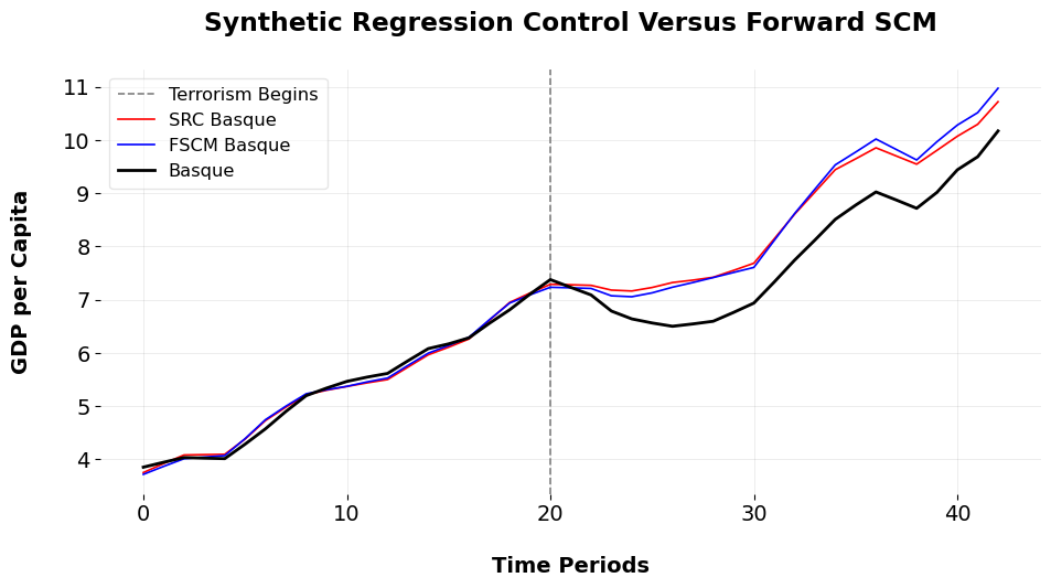
import pandas as pd
from mlsynth.mlsynth import SRC, FSCM
import matplotlib.pyplot as plt
import matplotlib

ubertheme = {
    "figure.facecolor": "white",
    "figure.figsize": (11,5),
    "figure.dpi": 100,
    "figure.titlesize": 16,
    "figure.titleweight": "bold",
    "lines.linewidth": 1.2,
    "patch.facecolor": "#0072B2",  # Blue shade for patches
    "xtick.direction": "out",
    "ytick.direction": "out",
    "font.size": 14,
    "font.family": "sans-serif",
    "font.sans-serif": ["DejaVu Sans"],
    "axes.grid": True,
    "axes.facecolor": "white",
    "axes.linewidth": 0.1,
    "axes.titlesize": "large",
    "axes.titleweight": "bold",
    "axes.labelsize": "medium",
    "axes.labelweight": "bold",
    "axes.spines.top": False,
    "axes.spines.right": False,
    "axes.spines.left": False,
    "axes.spines.bottom": False,
    "axes.titlepad": 25,
    "axes.labelpad": 20,
    "grid.alpha": 0.1,
    "grid.linewidth": 0.5,
    "grid.color": "#000000",
    "legend.framealpha": 0.5,
    "legend.fancybox": True,
    "legend.borderpad": 0.5,
    "legend.loc": "best",
    "legend.fontsize": "small",
}

matplotlib.rcParams.update(ubertheme)

# URL to fetch the dataset
url = 'https://raw.githubusercontent.com/jgreathouse9/mlsynth/refs/heads/main/basedata/basque_data.csv'
df = pd.read_csv(url)

treat = df.columns[-1]
time = df.columns[1]
outcome = df.columns[2]
unitid = df.columns[0]

config = {
    "df": df,
    "treat": treat,
    "time": time,
    "outcome": outcome,
    "unitid": unitid,
    "display_graphs": False,
    "counterfactual_color": "blue"
}

# Create instances of each model with the config dictionary
models = [SRC(config), FSCM(config)]


results = []
for model in models:
    result = model.fit()
    results.append((type(model).__name__, result))  # Store the model name and result as a tuple

plt.axvline(x=20, color='grey', linestyle='--', label="Terrorism Begins")

colors = ['red', 'blue']

for i, (model_name, result) in enumerate(results):
    counterfactual = result["Vectors"]["Counterfactual"]
    plt.plot(counterfactual, label=f"{model_name} Basque", linestyle='-', color=colors[i])

observed_unit = result["Vectors"]["Observed Unit"]
plt.plot(observed_unit, label=f"Basque", color='black', linewidth=2)

plt.xlabel('Time Periods')
plt.ylabel('GDP per Capita')
plt.title('Synthetic Regression Control Versus Forward SCM')
plt.legend()

plt.show()

Here we plot the counterfactuals for each method versus the observed donor units. The donor weights for the SRC are Aragon (0.044), Cantabria (0.13), Cataluna (0.241), Madrid (0.348), Navarra, Asturias (0.128), and Rioja (La) (0.104). These are not the same weights from the paper, since the paper incorporates the covariates from the orginal paper. In the paper, Austurias got 0.001, Cantabria got 0.311, Cataluna has 0.028, Madrid has 0.276, and La Rioja has 0.587. The ATT is -0.647, and the pre-treatment is 0.087. Forward SCM gets an ATT of -0.692 and an RMSE of 0.084. The FSCM algorithm selected 9 weights of the 16 donor units, Cataluna (0.826), Madrid (Comunidad De) (0.168), and Asturias (0.005). So, while the methods differ, they attain similar ATTs and reach similar practical conclusions. In the paper, the author also allows the donors to be screened via sure independent ranking and screening (PDF page 17). I didn’t implement this myself, but it seems to be a way to reduce the donor pool so that our estimates are improved because our donor pool has improved. I’ll include this as an option for SRC in the future, so users can implement it and maybe compare it to Forward Selection or the other methods mlsynth offers.

As ususal, email me with comments or questions, and share the post on LinkedIn should others find this helpful.