Maximizing value for business services and crafting effective public policy depends on knowing whether policies, promotions, new web features, taxes, or other interventions meaningfully affect metrics that we care about.
Researchers commonly use Difference-in-Differences designs and Synthetic Control methods (DID and SCM) to measure causal impacts.
DID requires \(\mathbb{E}[y_{1t}(0)] - \mathbb{E}[y_{\mathcal{N}_0 t}(0)] = \mathbb{E}[y_{1t-1}(0)] - \mathbb{E}[y_{\mathcal{N}_0 t-1}(0)]\), or parallel trends. Does not hold when the mean of controls is dissimilar to the trend of the treated unit/group.
SCM struggles when \(N_0>>T_0\), and is prone to overfitting in this setting. Also, smaller donor pools are preferable to mitigate interpolation biases. But picking a good donor pool can be challenging when there are very many controls.
While having all these is nice, they are all scattered in different libraries. They have different data structure demands, different options, and so on.
These approaches are very useful; they address high dimensional data structures via clustering/forward selection, allow for model selection between different SCM variants, address noisily observed outcomes, but many are either proprietary or not packaged, making the actual use of these estimators difficult.
Enter mlsynth…
The Python library mlsynth is meant to further democratize causal inference SC methods, each with different use cases.
At present it has roughly 20 different flavors of SCM.
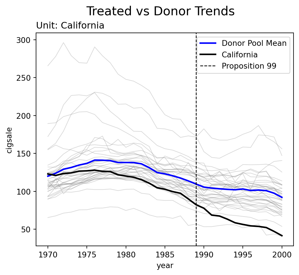
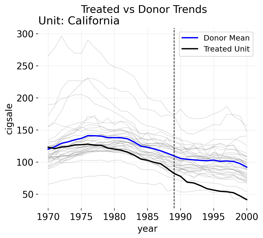
Parallel trends does not appear to hold for California with respect to its donor pool. California has a steeper downward sloping trend of cigarette consumption compared to the average of the donor pool. No matter what scalar constant we would shift the mean of the donor pool by, the mean difference would not be constant with respect to California. This suggests one of two solutions is viable: either parallel trends would hold with some control units, or we simply need to re-weight the donor pool to better match the pre-intervention trajectory.
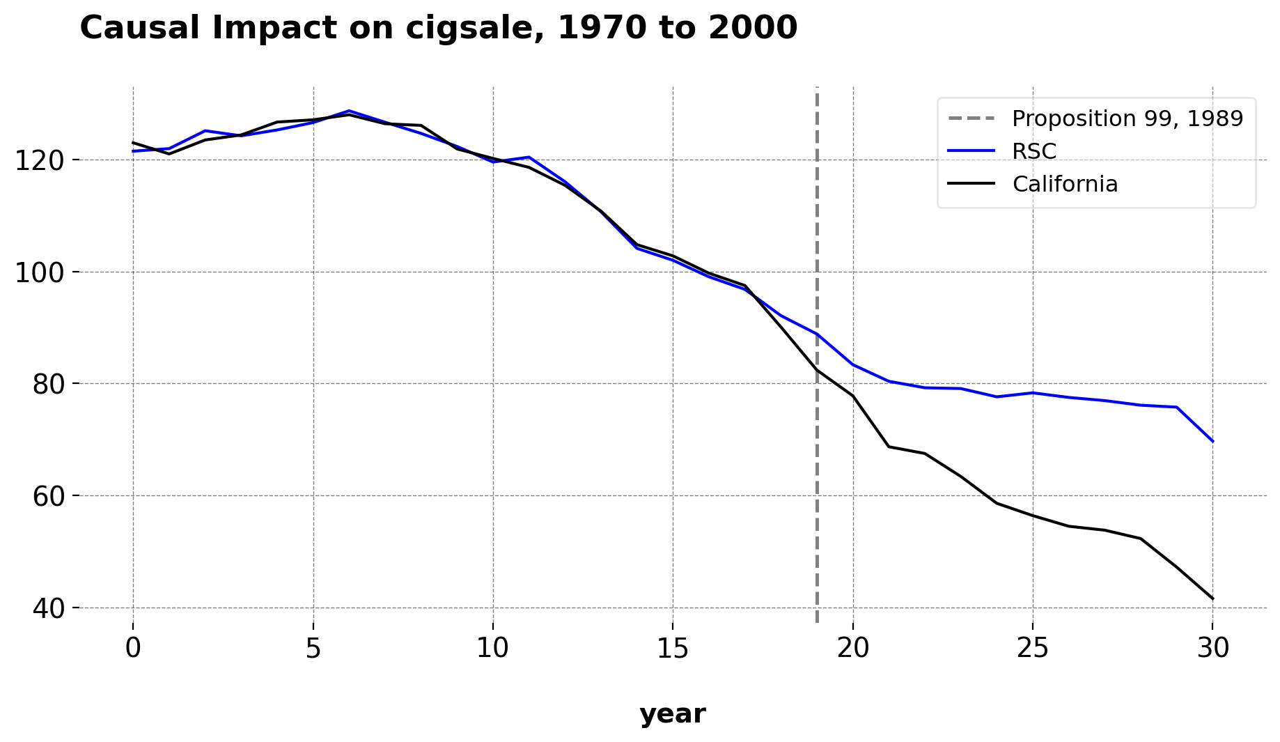
Here is the results of the CLUSTERSC class. This class implements the Robust Synthetic Control Method. We can see that this model fits the pre-treatment trajectory very well, without needing to use any of the seven covariates that the original paper uses.
Here, the weights are allowed to be negative and there is no summation constraint: PCA is used to denoise the donor pool, we select the number of singular values via a singular value thresholding, and we reconstruct the donor matrix to learn the weights via OLS. We may also use the Bayesian version of this estimator if we set Frequentist to False
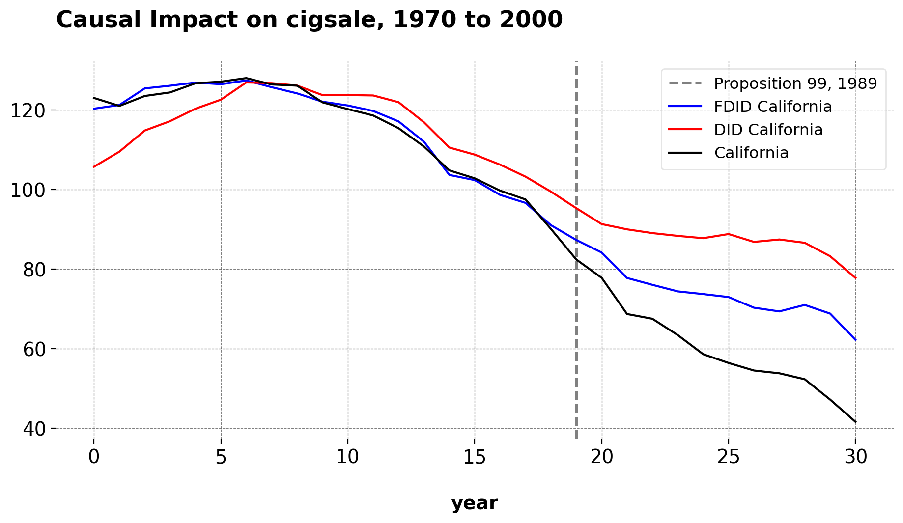
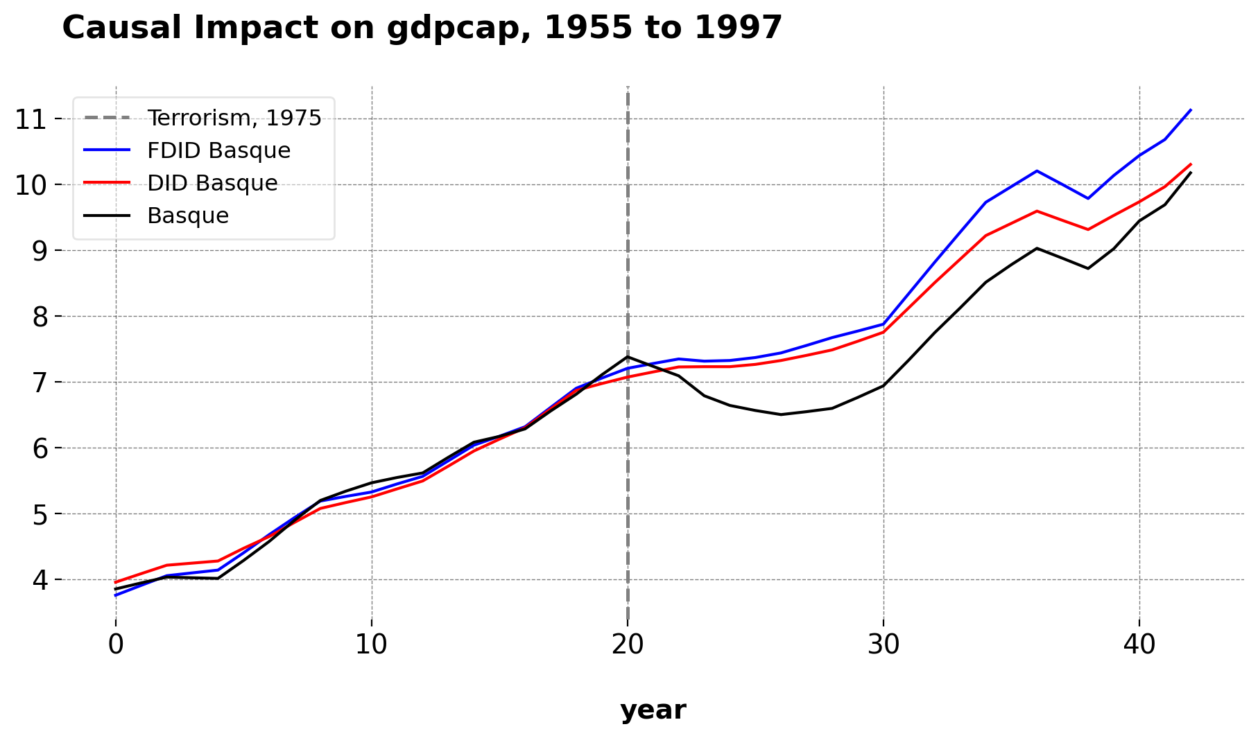
FDID is an iterative, data-driven approach that selects the control group for a treated unit.
By design, it is agnostic to which units to include or how many controls to use. The algorithm adds controls sequentially based on pre-treatment fit.
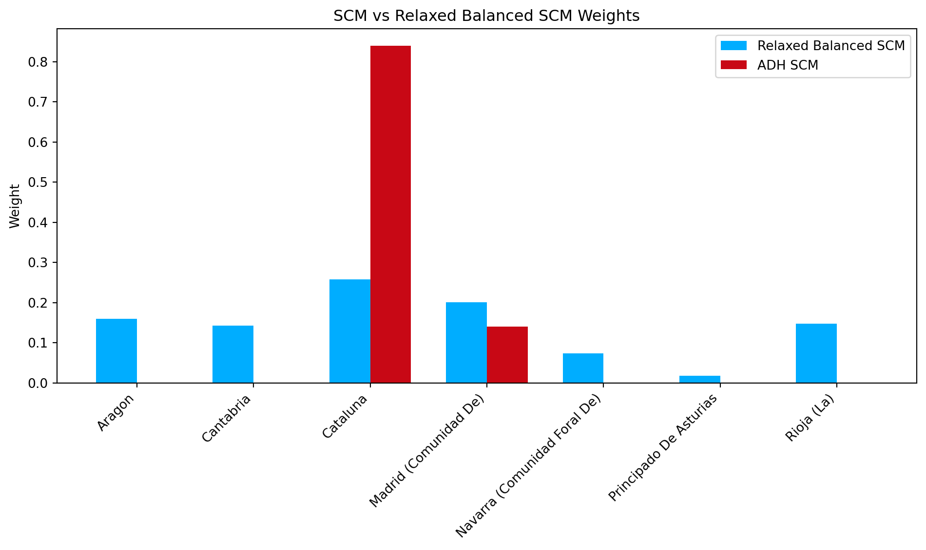
The ATT for ADH-SCM and the Relaxed Balanced SC are very similar, as is their pretreatment fits. However we can see that they select very different unit weights. The relaxed SC, with \(\tau\) chosen by cross validation, diversifies the prediction risk.
Aragon and Catalonia (weighted at 0.5), counterfactual similar to the relaxed SCM.
Simplicity of Use
Estimating multiple SCM/DID variants across different datasets requires only minimal changes to the API call (just the class name).
Furthermore, we can do this with essentially zero change in the data structure or input requirements beyond simple changes to a dictionary. Each .fit() call returns a comprehensive BaseEstimatorResults object containing treatment effects, fit diagnostics (e.g., RMSE, R-squared), time-series data, and (where applicable) donor weights, ready for analysis or visualization.
No manual data reshaping, cross-validation loops, or separate plotting functions are needed—mlsynth handles these under the hood.
Users can focus on the analysis, not on boilerplate preprocessing or plotting code.
mlsynth is also customizable. For advanced users, each class has its own configuration dictionary. To add a proprietary method, you can: