Shake it to the Max? Using the \(\ell_\infty\) norm for Synthetic Control Methods

Regularization in synthetic control methods has become an important econometric topic in recent years. Let \(\mathbf{y}_1 \in \mathbb{R}^{T_0}\) denote the pre-treatment outcomes for the treated unit and let \(\mathbf{Y}_0 \in \mathbb{R}^{T_0 \times |\mathcal{N}_0|}\) denote the corresponding donor matrix. In the most general terms, an SCM is a form of convex optimization where we use a set of donor units that were not exposed to a treatment to predict how the outcomes for a single (or set of) target unit(s) would have evolved without the treatment. In full generality, a synthetic control estimator solves the following family of programs:

\[ \mathbf{w} \;\in\; \underset{\mathbf{w} \in \mathcal{C}}{\operatorname*{argmin}} \; \mathcal{L}(\mathbf{Y}_0, \mathbf{y}_1, \mathbf{w}) \;+\; \mathcal{P}(\mathbf{w}), \]

subject to

\[ \mathcal{B}(\mathbf{Y}_0, \mathbf{y}_1, \mathbf{w}) \;\le\; \boldsymbol{\tau}. \]

Here \(\mathcal{L}(\cdot)\) denotes a data-dependent loss function governing pre-treatment fit, \(\mathcal{P}(\cdot)\) denotes a regularization or geometry-inducing penalty on the weights, and \(\mathcal{C}\) denotes a convex admissible set for the donor weights. The operator \(\mathcal{B}(\cdot)\) encodes balance or moment conditions, and \(\boldsymbol{\tau}\) controls the degree of relaxation. Either \(\mathcal{L}\) or \(\mathcal{B}\) may be identically zero, but not both. The classical synthetic control estimator of Abadie, Diamond, and Hainmueller is obtained by setting

\[ \mathcal{L}(\mathbf{Y}_0, \mathbf{y}_1, \mathbf{w}) = \left\| \mathbf{y}_1 - \mathbf{Y}_0 \mathbf{w} \right\|_2^2, \quad \mathcal{P}(\mathbf{w}) = 0, \quad \mathcal{B} \equiv 0, \]

with admissible weights given by

\[ \mathcal{C}_{\text{simplex}}:= \left\{ \mathbf{w} \in \mathbb{R}_{\geq 0}^{|\mathcal{N}_0|} : \mathbf{1}^\top \mathbf{w} = 1 \right\}. \]

In this case, balance is enforced entirely through the objective function.

Regularized Synthetic Control

Analysts have developed formulations of synthetic control that simultaneously account for level differences and control the geometry of the donor weights. To allow for level differences, we augment the donor matrix with an intercept term:

\[ \widetilde{\mathbf{Y}}_0 = \begin{bmatrix} \mathbf{Y}_0 & \mathbf{1} \end{bmatrix}, \qquad \widetilde{\mathbf{w}} = \begin{bmatrix} \mathbf{w} \\ b_0 \end{bmatrix}, \]

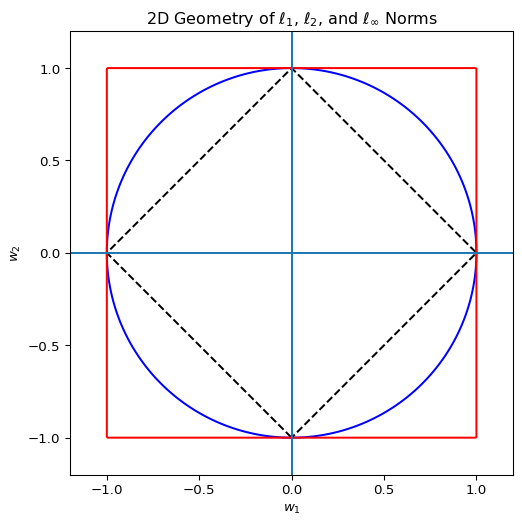
where \(b_0 \in \mathbb{R}\) captures an additive baseline shift. Regularization of the coefficients is also an important issue. Note that all penalties are applied to \(\mathbf{w}\), while \(b_0\) is left unpenalized. For a graphical example, see the plot:

import numpy as np
import matplotlib.pyplot as plt

# Grid for contour plots
x = np.linspace(-1.2, 1.2, 400)
y = np.linspace(-1.2, 1.2, 400)
X, Y = np.meshgrid(x, y)

# Norms
L1 = np.abs(X) + np.abs(Y)
L2 = np.sqrt(X**2 + Y**2)
Linf = np.maximum(np.abs(X), np.abs(Y))

plt.figure(figsize=(6, 6))

# Plot unit balls
plt.contour(X, Y, L1, levels=[1], colors="k", linestyles="dashed")
plt.contour(X, Y, L2, levels=[1], colors="blue")
plt.contour(X, Y, Linf, levels=[1], colors="red")

# Axes and aesthetics
plt.axhline(0)
plt.axvline(0)
plt.gca().set_aspect("equal", adjustable="box")
plt.xlim(-1.2, 1.2)
plt.ylim(-1.2, 1.2)

plt.title("2D Geometry of $\\ell_1$, $\\ell_2$, and $\\ell_\\infty$ Norms")
plt.xlabel("$w_1$")
plt.ylabel("$w_2$")

plt.show()

A common choice is the elastic net penalty, which encompasses a wide class of regularized SC estimators. These fit into the general framework by setting the balance operator \(\mathcal{B} \equiv 0\) (enforcing fit entirely through the objective, as in classical SCM), using a squared-error loss \(\mathcal{L}\) for pre-treatment fit, introducing a non-zero penalty \(\mathcal{P}\) to control weight geometry, and often relaxing the admissible set \(\mathcal{C}\) to allow greater flexibility (e.g., negative weights and no sum-to-one constraint, though variants may retain non-negativity for interpretability).

To allow for level differences, we augment the donor matrix with an intercept term:

\[ \widetilde{\mathbf{Y}}_0 = \begin{bmatrix} \mathbf{Y}_0 & \mathbf{1} \end{bmatrix}, \qquad \widetilde{\mathbf{w}} = \begin{bmatrix} \mathbf{w} \\ b_0 \end{bmatrix}, \]

where \(b_0 \in \mathbb{R}\) captures an additive baseline shift. The loss is then:

\[ \mathcal{L}(\mathbf{Y}_0, \mathbf{y}_1, \mathbf{w}, b_0) = \left\| \mathbf{y}_1 - \mathbf{Y}_0 \mathbf{w} - b_0 \mathbf{1} \right\|_2^2, \]

with \(\mathcal{B} \equiv 0\). Note that all penalties are applied only to \(\mathbf{w}\), while \(b_0\) is left unpenalized.

The first flavor, by Doudchenko and Imbens (2016), interpolates between the \(\ell_1\) norm and the \(\ell_2\) norm:

\[ \mathcal{P}(\mathbf{w}) = \lambda \Big( \alpha \lVert \mathbf{w} \rVert_1 + (1 - \alpha) \lVert \mathbf{w} \rVert_2^2 \Big), \qquad \alpha \in [0,1], \]

with \(\mathcal{C} = \left\{ \mathbf{w} \in \mathbb{R}^{|\mathcal{N}_0|}, b_0 \in \mathbb{R} \right\}\) (relaxing non-negativity and sum-to-one). The \(\ell_1\) term encourages sparsity (SC supported on few donors). Intermediate \(\alpha \in (0,1)\) yields the elastic net; special cases are \(\alpha = 1\) (pure LASSO) and \(\alpha = 0\) (pure Ridge).

Alternatively, as studied by Wang, Xing, and Ye (2025), one may replace the \(\ell_2\) term with the \(\ell_\infty\) norm:

\[ \mathcal{P}(\mathbf{w}) = \lambda \Big( \alpha \lVert \mathbf{w} \rVert_1 + (1 - \alpha) \lVert \mathbf{w} \rVert_\infty \Big), \qquad \alpha \in [0,1], \]

again with \(\mathcal{C} = \left\{ \mathbf{w} \in \mathbb{R}^{|\mathcal{N}_0|}, b_0 \in \mathbb{R} \right\}\). The \(\ell_\infty\) component caps the maximum absolute weight, producing a “balanced sparsity” effect: a small number of donors may be selected, but none dominates. When using the \(\ell_\infty\) variant of the elastic net, \(\alpha = 0\) corresponds to the pure max-norm penalty.

Geometrically, the \(\ell_1\)–\(\ell_\infty\) penalty replaces the circular ridge ball with a hyper-rectangular region, reflecting the analyst’s preference for bounding donor influence rather than merely smoothing it. These special cases highlight how the elastic net family interpolates continuously between sparsity and smoothness (or maximum weight control). Within the general framework, the optimization problem becomes:

\[ (\mathbf{w}, b_0) \;\in\; \underset{\mathbf{w} \in \mathbb{R}^{|\mathcal{N}_0|}, b_0 \in \mathbb{R}}{\operatorname*{argmin}} \; \mathcal{L}(\mathbf{Y}_0, \mathbf{y}_1, \mathbf{w}, b_0) + \lambda \Big( \alpha \lVert \mathbf{w} \rVert_1 + (1 - \alpha) \lVert \mathbf{w} \rVert_q \Big), \]

where \(q = 2\) recovers the standard elastic net (with \(\lVert \mathbf{w} \rVert_2^2\)) and \(q = \infty\) recovers the max-norm variant. Conceptually, the \(\ell_2\) term spreads weights smoothly while the \(\ell_\infty\) term limits any single donor’s dominance. This is analogous to a portfolio with position limits: no single donor can dominate the synthetic control, while overall weight distribution can be controlled via \(\alpha\) and \(\lambda\).

In practice, this can be important: in the original 2003 SCM paper, the donors Catalonia and Madrid received weights of 0.8508 and 0.1492, respectively. While this allocation makes sense economically, there are settings where analysts may wish to reduce the influence of any single donor.

A Relaxed Balanced Approach

Other approaches to mitigating high-dimensionality are possible. Liao, Shi, and Zheng (2025), introduce a relaxation of the fit conditions imposed by the elastic net estimators above. Here, the loss is set to zero, a penalty is placed on the weights, and fit is enforced via a constraint

\[ (\mathbf{w},\gamma) \in \underset{ \substack{ \mathbf{w}\in\mathbb{R}^{|\mathcal{N}_0|}_+,\\[2pt] \mathbf{1}^\top\mathbf{w}=1,\;\gamma\in\mathbb{R} } }{\operatorname*{argmin}} \;\; \|\mathbf{w}\|_2^2 \quad \text{s.t.} \quad \left\| \mathbf{G}\mathbf{w} - \mathbf{a} + \gamma\mathbf{1} \right\|_\infty \le \tau, \qquad \mathbf{G} = \frac{1}{T_0}\mathbf{Y}_0^\top\mathbf{Y}_0, \quad \mathbf{a} = \frac{1}{T_0}\mathbf{Y}_0^\top\mathbf{y}_1. \]

The slack variable \(\gamma\) shifts all donor projections uniformly and is estimated jointly with \(\mathbf{w}\), allowing small, evenly distributed violations when exact pre-treatment matching is infeasible. Alternative penalties can also be used: negative entropy

\[ (\mathbf{w},\gamma) = \underset{ \substack{ \mathbf{w}\in\mathbb{R}_+^{|\mathcal{N}_0|},\\ \mathbf{1}^\top\mathbf{w}=1,\;\gamma\in\mathbb{R} } }{\operatorname*{argmin}} \left[ \sum_{j} w_j \log w_j \right] \quad \text{s.t.}\quad \big\|G w - a + \gamma\mathbf{1}\big\|_\infty \le \tau. \]

encourages dense allocation, while empirical likelihood

\[ (\mathbf{w},\gamma) = \underset{ \substack{ \mathbf{w}\in\mathbb{R}_+^{|\mathcal{N}_0|},\\ \mathbf{1}^\top\mathbf{w}=1,\;\gamma\in\mathbb{R} } }{\operatorname*{argmin}} \left[ -\sum_{j} \log w_j \right] \quad \text{s.t.}\quad \|G w - a + \gamma\mathbf{1}\|_\infty \le \tau. \]

discourages zero weights. In all cases, the constraint enforces relaxed balance, while the penalty governs the weight structure.

This contrasts with classical SCM and elastic net approaches. There, fit is minimized in the objective and the weights absorb all discrepancies. In the relaxed balance method, fit is a constraint, the objective imposes an \(\ell_2\) (or other) penalty on the weights, and \(\gamma\) allows controlled relaxation—analogous to portfolio optimization with position limits, where constraints cap exposure to any single asset while the objective encourages diversification or avoidance of zero positions. This separation is particularly useful in high-dimensional donor pools or when robustness to over-reliance on any single donor is desired.

An Example in mlsynth

As usual, these may be implemented in mlsynth, using the RESCM class. To install mlsynth, you must have Github on your machine and and do

pip install -U git+https://github.com/jgreathouse9/mlsynth.git

from the command line or within your virtual Python environment. To run the model, users provide a panel data frame along with the outcome variable, a treatment indicator, a unit identifier, and a time variable. Optional configuration includes whether to display plots, save results, and customize the colors of treated and counterfactual series are also present.

Modeling options are controlled via the models_to_run dictionary, where a run: bool specifies whether the model is estimated. Relaxed SCM estimators are specified by the "RELAXED" key, with the type of relaxation chosen through the relaxation parameter. Options include l2 for standard Euclidean relaxation, entropy for entropy-based relaxation, and el for empirical likelihood relaxation. The relaxation strength is controlled by the tau parameter, which can be provided explicitly (in which case no cross-validation is performed) or selected via cross-validation over a grid of candidate values. The number of candidate taus is controlled by n_taus, and the number of cross-validation folds by n_splits.

Elastic Net SCM estimators are specified by the "ELASTIC" key and combine L1 with either \(\ell_2\) or \(\ell_\infty\) penalties on donor weights via enet_type="L1_L2" or enet_type="L1_INF". The alpha parameter controls the mixture between L1 and the second norm, while lambda controls the overall penalty strength. If lambda is zero, no cross-validation is performed. If lambda is provided but alpha is not, cross-validation is performed over alpha, and vice versa. An optional intercept can be added via fit_intercept.

The feasible set for the donor weights is specified via the constraint_type parameter. Users may select unit, simplex, affine, nonneg, or unconstrained. These are defined as follows:

\[ \begin{aligned} \mathcal{C}_{\text{unit}} &:= \left\{ \mathbf{w} \in [0,1]^{|\mathcal{N}_0|} \right\}\\[6pt] \mathcal{C}_{\text{simplex}} &:= \left\{ \mathbf{w} \in \mathbb{R}_{\geq 0}^{|\mathcal{N}_0|} : \mathbf{1}^\top \mathbf{w} = 1 \right\}\\[6pt] \mathcal{C}_{\text{affine}} &:= \left\{ \mathbf{w} \in \mathbb{R}^{|\mathcal{N}_0|} : \mathbf{1}^\top \mathbf{w} = 1 \right\}\\[6pt] \mathcal{C}_{\text{nonneg}} &:= \mathbb{R}_{\geq 0}^{|\mathcal{N}_0|}\\[6pt] \mathcal{C}_{\text{unconstrained}} &:= \mathbb{R}^{|\mathcal{N}_0|} \end{aligned} \]

The unit constraint restricts each weight to the unit interval independently. This forces the synthetic control to be a strict interpolation with bounded contributions—no single donor can contribute more than 100%, making it the most conservative option that completely rules out extrapolation while providing highly interpretable, share-like weights. The classical simplex constraint requires non-negative weights that sum to one. The synthetic control is therefore a convex combination of the donors, lying inside or on the boundary of their convex hull. This setting offers excellent interpretability (weights resemble portfolio shares or probabilities) and prohibits any extrapolation, which is why it remains the default choice in most applied synthetic control studies. The affine constraint relaxes non-negativity but retains the sum-to-one requirement. It allows negative weights, meaning the synthetic control can lie outside the convex hull while staying within the affine subspace spanned by the donors. This introduces controlled extrapolation (useful when the treated unit has a different level or trend but shares parallel paths), but at the cost of reduced interpretability, as negative weights imply “subtracting” the contribution of certain donors. The nonneg constraint permits any non-negative weights without normalization. The synthetic control can lie far outside the convex hull along positive directions (conic extrapolation), which can substantially improve pre-treatment fit in some cases, though the lack of scaling makes the weights harder to interpret economically. Finally, the unconstrained option imposes no restrictions whatsoever, allowing signed weights of any magnitude. This grants maximum flexibility and typically yields the best pre-treatment fit (as in most elastic-net or machine-learning-style SCMs), but it also permits unrestricted extrapolation and offers the lowest interpretability, with weights often lacking direct economic meaning.

Relaxation methods like entropy and el are simplex weights by definition. Once the configuration is set, calling RESCM(config).fit() estimates the selected models on the pre-treatment period and produces counterfactual predictions for both pre- and post-treatment periods. The output is an EstimatorResults object containing separate results for relaxed and elastic SCMs (depending on what the user specifies), including donor weights, time series of observed and counterfactual outcomes, and fit diagnostics such as pre- and post-treatment RMSE. To date, this is the most flexible class of estimators mlsynth provides.

Application

Now for an empirical application for the Basque Country. First I load the data and set up the model

import pandas as pd
import matplotlib.pyplot as plt
from mlsynth import RESCM
from IPython.display import display, Markdown

url = "https://raw.githubusercontent.com/jgreathouse9/mlsynth/refs/heads/main/basedata/basque_data.csv"
data = pd.read_csv(url)

base_config = {
    "df": data,
    "outcome": data.columns[2],
    "treat": data.columns[-1],
    "unitid": data.columns[0],
    "time": data.columns[1],
    "display_graphs": False,
    "save": False,
    "counterfactual_color": ["blue", "red"]
}


relax_types = ["l2", "entropy", "el"]
results = {}

for rtype in relax_types:

    config = {
        **base_config,
        "models_to_run": {
            "RELAXED": {
                "run": True,
                "relaxation": rtype,
                "tau": None,
                "n_taus": 100
            }
        }
    }

    arco = RESCM(config).fit()

    results[f"RELAXED_{rtype}"] = {
        "counterfactual": arco.relax.time_series.counterfactual_outcome,
        "weights": arco.relax.weights.donor_weights,
        "method": arco.relax.method_details.method_name,
        "tau": arco.relax.method_details.parameters_used['tau_used']
    }

config_l1l2 = {
    **base_config,
    "models_to_run": {
        "ELASTIC": {
            "run": True,
            "constraint_type": "unit",
            "intercept": False,
            "enet_type": "L1_L2"
        }
    }
}

arco_l1l2 = RESCM(config_l1l2).fit()

results["ELASTIC_L1_L2"] = {
    "counterfactual": arco_l1l2.elastic.time_series.counterfactual_outcome,
    "weights": arco_l1l2.elastic.weights.donor_weights,
    "method": arco_l1l2.elastic.method_details.method_name
}

config_l1linf = {
    **base_config,
    "models_to_run": {
        "ELASTIC": {
            "run": True,
            "constraint_type": "unit",
            "intercept": False,
            "enet_type": "L1_INF"
        }
    }
}

arco_l1linf = RESCM(config_l1linf).fit()

results["ELASTIC_L1_LINF"] = {
    "counterfactual": arco_l1linf.elastic.time_series.counterfactual_outcome,
    "weights": arco_l1linf.elastic.weights.donor_weights,
    "method": arco_l1linf.elastic.method_details.method_name
}


weights_df = pd.DataFrame({
    name: pd.Series(res["weights"])
    for name, res in results.items()
}).round(3)


# ---------------- Display as Markdown ----------------
markdown_table = weights_df.to_markdown()

/opt/hostedtoolcache/Python/3.13.12/x64/lib/python3.13/site-packages/mlsynth/utils/optutils.py:174: UserWarning:

Solution may be inaccurate. Try another solver, adjusting the solver settings, or solve with verbose=True for more information.

/opt/hostedtoolcache/Python/3.13.12/x64/lib/python3.13/site-packages/mlsynth/utils/optutils.py:174: UserWarning:

Solution may be inaccurate. Try another solver, adjusting the solver settings, or solve with verbose=True for more information.

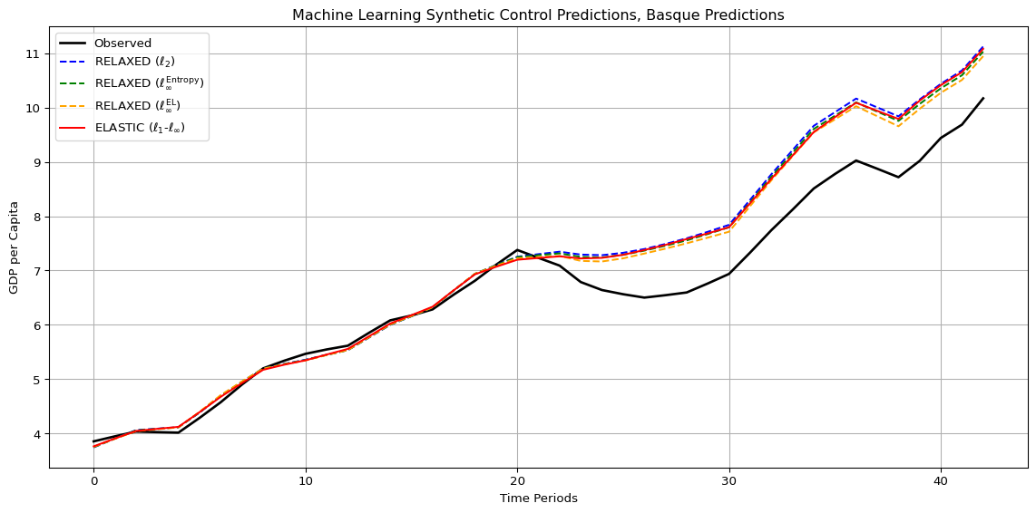
The synthetic control hyper-parameters (tau, alpha, and lambda) were tuned via time-series cross validation. For the elastic net methods, two variants were considered: \(\alpha \ell_1 + (1-\alpha) \ell_\infty\) and \(\alpha \ell_1 + (1-\alpha) \ell_2\). Both employed 4-fold time series cross-validation with standardized donor predictors. As we eiscussed above for the elastic net models, the alpha parameter governs the trade-off between sparsity and the secondary norm. For both variants, this was was approximately 0.554, while the lambda parameter controlling overall regularization strength was around 0.084 for the \(\ell_1+\ell_\infty\) variant and 0.128 for the \(\ell_1+\ell_2\) variant. I used affine weights for both of these. For the relaxed balanced synthetic control variants—\(\ell_2\) relaxation, empirical likelihood, and entropy relaxation—the slack parameter \(\tau\) was set to approximately 0.00262 for all three. This small value enforces tight balance, encouraging the synthetic control to match pre-treatment outcomes closely while allowing minimal flexibility to stabilize the optimization and prevent extreme weight concentration. This was also tuned by the same cross validation method as above, and you can see my Python code for the sklearn details.

# ---------------- Plotting ----------------

plt.figure(figsize=(12, 6))

observed = arco_l1linf.elastic.time_series.observed_outcome
t = range(len(observed))

plt.plot(t, observed, color="black", linewidth=2, label="Observed")

styles = {
    "RELAXED_l2": "--",
    "RELAXED_entropy": "--",
    "RELAXED_el": "--",
    "ELASTIC_L1_L2": "-",
    "ELASTIC_L1_LINF": ":"
}

for name, res in results.items():
    plt.plot(t, res["counterfactual"], linestyle=styles[name], label=res["method"])

plt.title("Basque Country, Synthetic Controls")
plt.xlabel("Time")
plt.ylabel("GDP per Capita")
plt.legend()
plt.grid(True)
plt.tight_layout()
plt.show()

Here are the weights:

display(Markdown(markdown_table))

	RELAXED_l2	RELAXED_entropy	RELAXED_el	ELASTIC_L1_L2	ELASTIC_L1_LINF
Andalucia	0	0	0.012	0	0
Aragon	0.176	0.132	0.047	0	0.263
Baleares (Islas)	0	0.005	0.009	0	0
Canarias	0	0	0.007	0	0
Cantabria	0.127	0.087	0.035	0	0
Castilla Y Leon	0	0.007	0.016	0	0
Castilla-La Mancha	0	0	0.008	0	0
Cataluna	0.289	0.387	0.621	0.53	0.239
Comunidad Valenciana	0	0.004	0.015	0	0
Extremadura	0	0	0.013	0	0
Galicia	0	0	0.01	0	0
Madrid (Comunidad De)	0.206	0.177	0.107	0.067	0.143
Murcia (Region de)	0	0.01	0.015	0	0
Navarra (Comunidad Foral De)	0.037	0.04	0.024	0	0
Principado De Asturias	0	0.028	0.022	0.115	0.102
Rioja (La)	0.166	0.121	0.04	0.288	0.252

Across all model variants (elastic net and relaxed balanced synthetic control alike) the donor weights exhibit a high degree of stability in which regions matter, even though the regularization structure changes how weight mass is distributed. In particular, Catalonia consistently receives the largest or among the largest weights, regardless of whether the method emphasizes sparsity (\(\ell_1\)-based elastic nets), smoothness (\(\ell_2\) relaxation), or dispersion (entropy relaxation). This is intuitive: Catalonia shares a closely related political and economic trajectory with the Basque Country, including early industrialization, strong regional identity, and similar exposure to national and international economic forces. In the outcome space, it is therefore unsurprising that Catalonia emerges as the closest synthetic analog. Beyond Catalonia, a recurring set of regions (La Rioja, Cantabria, and Navarre) also receive nontrivial weights across specifications. These regions are literal geographic neighbors of the Basque Country, sharing labor markets, trade linkages, and historical development patterns. Their repeated appearance across models suggests that geographic proximity aligns well with similarity in pre-treatment outcomes, reinforcing the idea that the optimization is recovering economically meaningful structure rather than exploiting numerical artifacts. Aragon also consistently enters the synthetic control, despite not bordering the Basque Country directly. Its location in northern Spain and its intermediate economic profile make it a plausible contributor, particularly under methods that allow moderate dispersion of weights. Finally, Madrid receives a positive—though typically smaller—weight across most specifications. While geographically distant, Madrid’s role as the national capital and its high level of wealth and development make it a natural partial comparator, especially in models that permit signed or less restrictive weighting schemes.

In the original SC solution, the donor weights were highly concentrated, with weights of 0.8508 and 0.1492 of Catalonia and Madrid respectively. This extreme concentration is a well-known feature of canonical SCM: when the feasible set is restricted to the simplex and no explicit regularization is imposed, the optimizer is free to place nearly all mass on the single donor that best matches the treated unit in the pre-treatment outcome space. In this sense, the original weights represent a corner solution driven almost entirely by fit, with little incentive to distribute weight more broadly across similar regions. Introducing a max-norm–based component (either explicitly via an \(\ell_\infty\) penalty or implicitly through relaxed balance constraints) fundamentally changes this behavior. The \(\ell_\infty\) norm directly penalizes the largest coefficient, which has the effect of tempering the size of dominant weights. Rather than allowing Catalonia to absorb nearly all the mass, the optimization trades a small amount of fit for a substantial reduction in the maximum weight. As a result, weight is redistributed toward nearby or economically similar regions (such as La Rioja, Cantabria, Navarre, and Aragon) while still preserving Catalonia’s central role in the counterfactual. Importantly, this redistribution is not arbitrary: it occurs along economically meaningful dimensions already latent in the data. This tempering effect operates in both the fit space and the balance space. In the fit space, the max norm discourages over-reliance on a single donor to track pre-treatment outcomes perfectly, leading to a smoother approximation that averages across multiple close matches. In the balance space, the \(\ell_\infty\) constraint limits the extent to which any single donor can shoulder the burden of matching outcomes, thereby encouraging broader participation in satisfying the balance conditions. The result is a synthetic control that is less brittle and less sensitive to idiosyncratic noise in any one donor unit.

Crucially, this moderation does not overturn the substantive story. Catalonia remains the dominant contributor across specifications, reflecting its strong historical, political, and economic similarity to the Basque Country. Madrid continues to receive a positive but secondary weight, consistent with its role as the national capital and a benchmark for economic development. What changes under the max norm is not who matters, but how much any single region is allowed to matter. In this way, the authors frame their resepctive \(\ell_\infty\) norm strucures as a principled mechanisms for controlling concentration of weights in high-dimensional setting, yielding weights that are more evenly distributed, more stable, and arguably more credible, while still preserving the core economic relationships identified by the original SCM.

Conclusion

As usual, you’re free to inspect my code for this methodology and give any feedback you wish. I have been busy lately, so I’ve not been able to develop mlsynth as much as I’ve wanted to. But either way, this represents a really interesting way to regularize sythethic control methods, and the RESCM class represents how I plan to work with these methods going forward.