9 Difference-in-Differences
Note
For the below, let \(i\) index the units and \(t\) index all time periods. \(\mathcal{N}_0\) is the control group, where \(i=1\) is the singular treated unit.
Even though we cannot randomize all treatments/policies, does this mean that we cannot do policy analysis at all? No. Modern econometrics has developed a slew of methods for doing policy analysis when the intervention of interest simply cannot be subject to a controlled experiment in Stata, R, and Python. I now introduce the difference-in-differences method (DD), using Proposition 99 as an example case. DD is a method used for panel data, where we observe multiple units over many periods of time.
9.1 Underlying Theory of DD
DD is predicated on the idea that we may use the average of our controls as a comparison for one or more treated units. That is, it assumes our outcomes are generated by some time specific effect and some unit specific effect, \[ y_{it}= a_i + b_t \]
where \(a_i\) is the unit specific effect (note the \(i\) indexer for \(a\)) and \(b_t\) is the time effect. The unit component \(a_i\) is the unit-stable effect of factors that affect the outcome. We ususally do not expect for these to vary much over time. Examples of unit stable factors include things like culture, geography, hidden/latent economic conditions and aspects we cannot as easily observe. As one of my instructors once said in his thick Kentucky accent, “there is something that makes Alabama, Alabama.” By contrast, the time effect \(b_t\) is a time-shock. These are things which we expect to vary across time, but affect the units similarly, such as economic depressions, holidays, or other things we expect to be time-stable, unit variant. The summation of these two factors produces our outcomes, which we econometricians call the two-way fixed effects model.
For DD, units with similar contextual factors will on average be more comaprable in terms of their trends (we will formalize a definition of this more below). For example, suppose we wish to study the impact of the Maui wildfires on the seasonally adjusted level of tourism. A natural control group for Maui might be Hawai’i, O’ahu, Moloka’i, Lana’i, and Kaua’i. All of these islands may have different levels of tourism. However, due to their relatively similar cultural history and other contextual factors, it may make sense that these islands would serve as a better counterfactual to Maui than say, Honshu, Japan or Palma de Mallorca, since places with the same contextual factors will likely have simialr trends to one another. In other words, due to their baseline similarities, it is more likely that the average trends of these control group islands would move similarly to the Maui, if the fires did not happen. And, if this is true, all we need to do then is estimate whatever the time-differences are between Maui and the control group.
9.1.1 Introducing Parallel Trends
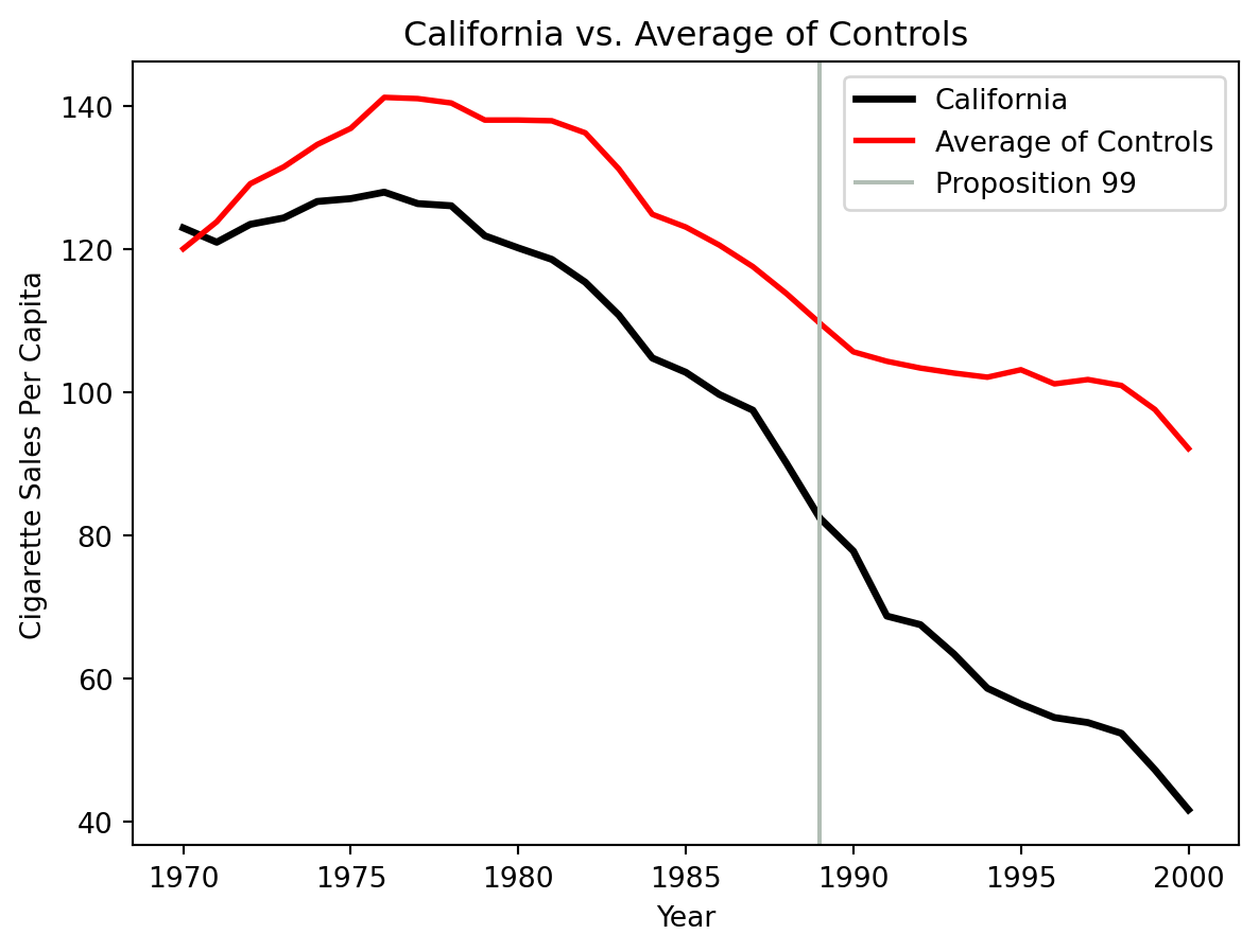
We can begin by graphing the trends of our control unit and the trend of the average of controls.
Here, we plot the cigarette consumption of California versus the average of control states. We can see in 1970, California is fairly similar to the control average. In fact, the average of controls and California both grow in their consumption rates up until 1976. However as the years progress, the average trend of controls grows at a much faster rate than California’s. California’s smoking trends grew relatively little and begin to precipitously fall in and after 1976, whereas the control group’s trend has much higher rates of smoking. The way to make this plot in Stata would be
clear *
cls
u "https://github.com/jgreathouse9/FDIDTutorial/raw/main/smoking.dta", clear

keep year id cigsale

qui reshape wide cigsale, i(year) j(id)

order cigsale3, a(year)

egen ymean = rowmean(cigsale1-cigsale39)

line cigsale3 ymean year
Either way, we can see that there is a difference between all 38 controls and California when we plot it. But again that’s okay: what if we do not need the means to be balanced exactly? What if we just need for the trends of the groups to be similar enough to one another? DD asks us, as analysts, to accept a singular condition as plausible: namely, that the intercept (time trend) adjusted average of our controls is a good enough proxy for how the treated unit’s outcomes would look absent treatment. This is called the “parallel trends assumption”.
Definition 9.1 (Parallel Trends) The parallel trends assumption says that the difference between the treated group and the control group would have been constant absent the treatment, or \(\hat{y}_{1t}^0-\bar{y}_{\mathcal{N}_0t}=\hat\alpha_{\mathcal{N}_0}+ \epsilon\).
PTA means that if the intervention never happened, the counterfactual would move in the same way as the average trend of our control group. A good first step to this is simply plotting the trajectory of the treated unit and the averge of controls. However, PTA is inherently untestable globally. Since we only actually observe units as treated or not due to the switching equation, \(y_{it}=d_{it}y^{1}_{it}+\left(1-d_{it} \right)y^0_{it}\), it is ultimately a statement about the counterfactual. So, as a result, the key we shall focus on is the parallel-ness in the pre-intervention period, since this is the only time period we observe all of our units without treatment. To put it a slightly different way, PTAs generally posit that history is the guide to the future: if the control group’s trend behaves similarly to the treated unit in the past, on average, then we simply use this as an extrapolation for the future trend of the treated unit.
For DD, we need at least one treated unit, one control unit, one before period, and one after period (though of course, we may have many pre-treatment periods, and many treated units) Roth et al. (2023). For our purposes, the simplest possible setup is the case where we have exactly one control unit, one treated unit, and more than one pre and post intervention time period. Let’s just look at how the trends of individual controls compares to single control units.
clear *

qui foreach x of numlist 13 10 2 39 38 7 14 4 17 26 27 34 31 5  {

cls
u "https://github.com/jgreathouse9/FDIDTutorial/raw/main/smoking.dta", clear


loc newstate = `x'

levelsof state if id ==`newstate', loc(cstate) clean

qui {
keep id year cigsale

qui reshape wide cigsale, j(id) i(year)

order cigsale3, a(year)
tempvar ymeangood ydiff ymean cf te
egen `ymean' = rowmean(cigsale`newstate')

}

*** Normal DID, all controls

g `ydiff' = cigsale3-`ymean'
reg `ydiff' if year < 1989


loc alpha = e(b)[1,1] // here is the intercept shift

g `cf' = `ymean' + `alpha' // DID Counterfacutal


twoway (connected cigsale3 year if year , mcolor(black) msize(small) msymbol(smcircle) lcolor(black) lwidth(medthick)) ///
    (connected cigsale`newstate' year, mcolor(gs11) msize(small) msymbol(smsquare) lcolor(gs11) lpattern(solid) lwidth(thin)), ///
    ylabel(#10, grid glwidth(vthin) glcolor(gs8%20) glpattern(dash)) ///
    xline(1989, lwidth(medium) lpattern(solid) lcolor(black)) ///
    xlabel(#10, grid glwidth(vthin) glcolor(gs8%20) glpattern(dash)) ///
    legend(cols(1) ///
    position(7) ///
    order(1 "California" 2 "`cstate'") ///
    region(fcolor(none) lcolor(none)) ring(0)) ///
    scheme(sj) ///
    graphregion(fcolor(white) lcolor(white) ifcolor(white) ilcolor(white)) ///
    plotregion(fcolor(white) lcolor(white) ifcolor(white) ilcolor(white)) ///
    name(badplot`x', replace) yti(Cigarette Sales) ti("`cstate' as a Control")

}
Nothing crazy is happening here. I’ve just plotted the trend of California versus the tobacco consumption trends of a few randomly selected controls. Now, we will begin to consider testing for parallel trends in the pre-intervention period, with each control unit. One way of doing this, and there are others, is by simply using OLS. Consider the definition of PTA above, where the following equation holds: \(\hat{y}_{1t}^0-\bar{y}_{\mathcal{N}_0t}=\hat\alpha_{\mathcal{N}_0}+ \epsilon\). Notice anything funny about this equation? Well… We can actually estimate this as a linear regression model, where we only have one variable!
Why?
Here is the definition of PTA: \(\hat{y}_{1t}^0-\bar{y}_{\mathcal{N}_0t}=\hat\alpha_{\mathcal{N}_0}+ \epsilon\). We can calculate \(\bar{y}_{\mathcal{N}_0t} = \frac{1}{|\mathcal{N}_0|} \sum_{i \in \mathcal{N}_0} y_{it}\), or the control group average. Here, \(|\mathcal{N}_0|\) is the number of control units (what we call the cardinality of a discrete set in mathemtics, using the absolute value symbol), and the overbar means that we are calculating the sample mean. For this univariate regression model, we simply subtract (or, demean) the control group average from the treated unit is outcomes. Let this demeaned \(y_{1t}\) be denoted as \(\tilde{y}_{1t}=y_{1t}-\bar{y}_{\mathcal{N}_0t}\) We then estimate the regression model \(\tilde{y}_{1t}=\hat\alpha_{\mathcal{N}_0}+ \epsilon\). Our variable of interest here is simply the demeaned value of the treated outcomes, and we are in effect estimating the constant.
To connect this to OLS, DD seeks the value of the \(\alpha\) (the constant) which minimizes the distance between the control group and the treated unit. Here we do this with multiple plots, using a single control unit.
clear *

// DID one control each unit

qui foreach x of numlist 22 13 2 7  17 27 26 39 14 5 31 38 10  34  4 19 {

cls
u "https://github.com/jgreathouse9/FDIDTutorial/raw/main/smoking.dta", clear


loc newstate = `x'

levelsof state if id ==`newstate', loc(cstate) clean

qui {
keep id year cigsale

qui reshape wide cigsale, j(id) i(year)

order cigsale3, a(year)

tempvar ymeangood ytilde ymean cf te rss tss

egen `ymean' = rowmean(cigsale`newstate')

}

g `ytilde' = cigsale3-`ymean' // here is the demeaning step I mention above

reg `ytilde' if year < 1989 // univariate regression


loc alpha = e(b)[1,1] // here is the intercept shift

// this step above gives us the intercept shift that

// corresponds to the average differnece between California and
// the single treated unit


g `cf' = `ymean' + `alpha' // DID Counterfacutal

qui summarize cigsale3 if year < 1989, mean
local mean_observed = r(mean)

* Calculate the Total Sum of Squares (TSS)
qui generate double `tss' = (cigsale3 - `mean_observed')^2 if year < 1989
qui summarize `tss' if year < 1989
local TSS = r(sum)


* Calculate the Residual Sum of Squares (RSS)
qui generate double `rss' = (cigsale3 - `cf')^2 if year < 1989 //pre period r2
qui summarize `rss' if year < 1989
local RSS = r(sum)


loc r2 = 1 - (`RSS' / `TSS')


twoway (connected cigsale3 year if year , mcolor(black) msize(small) msymbol(smcircle) lcolor(black) lwidth(medthick)) ///
    (connected cigsale`newstate' year, mcolor(gs11) msize(small) msymbol(smsquare) lcolor(gs11) lpattern(solid) lwidth(thin)) ///
    (connected `cf' year, mcolor(gs11) msize(small) msymbol(smtriangle) lcolor(gs11) lwidth(thin)), ///
    ylabel(#10, grid glwidth(vthin) glcolor(gs8%20) glpattern(dash)) ///
    xline(1989, lwidth(medium) lpattern(solid) lcolor(black)) ///
    xlabel(#10, grid glwidth(vthin) glcolor(gs8%20) glpattern(dash)) ///
    legend(cols(1) ///
    position(7) ///
    order(1 "California" 2 "`cstate'" 3 "DID California") ///
    region(fcolor(none) lcolor(none)) ring(0)) ///
    scheme(sj) ///
    graphregion(fcolor(white) lcolor(white) ifcolor(white) ilcolor(white)) ///
    plotregion(fcolor(white) lcolor(white) ifcolor(white) ilcolor(white)) ///
    name(plot`x', replace) yti(Cigarette Sales) ti("`cstate' as a Control: R2 = `r2'") ///
    subti(alpha: `alpha')

}
This code estimates a one unit DD model, using various different states as the single control unit. Again for emphasis, the alpha term is the time-fixed effect as I described above. The control unit, in this case, is the proxy for the unit fixed effect, or the latent factors that generate the outcome. I begin with New Hampshire and Kentucky. We can see that these controls are clearly not parallel to California in the pre 1989 period. Why not? Well… their trends are not similar. New Hampshire’s trend of tobacco consumption is plummeting relative to California in the pre-1989 period. Its trends of tobacco consumption were also increasing by a lot in the pre-treatment period relative to California. It even has a negative R-squared statistic, meaning it harms our ability to predict the sales trends for California.
Kentucky also has a negative R-squared. Its consumption trends rise a lot into the 1970s, and decline at a slower rate than California’s. When we look at the DD California (which is literally just New Hamphshire/Kentucky minus \(\alpha\) (alpha from the code), we see that the predictions (the line with the triangles) does not line up very well with California before 1989. Now… fast forward to the very end of the graph window in Stata, looking at plot19. See the state of Montana? Its consumption trend, when shifted by an intercept, does well at explaining the pre-intervention trend of California.
See how while even though their trends are not 100% the same, they are similar? Plot4, for Colorado, does the same, also appearing to fit California well in the pre policy period. To illustrate this more, consdider what would happen if we used two poor controls, Kentucky and New Hampshire
Here is the worse plot (NH + Kentucky)
clear *
cls
u "https://github.com/jgreathouse9/FDIDTutorial/raw/main/smoking.dta", clear

// NH Kentucky
xtdescribe

loc newstate = 13 // 13 =Kentucky

qui levelsof state if id ==`newstate', loc(cstate) clean

qui {
keep id year cigsale

qui reshape wide cigsale, j(id) i(year)

order cigsale3, a(year)
egen ymean = rowmean(cigsale22 cigsale13)
}

cls

*** DID, bad controls

g ydiff = cigsale3-ymean

reg ydiff if year < 1989


loc alpha = e(b)[1,1] // here is the intercept shift

g cf = ymean + `alpha' // DID Counterfacutal

tempvar tss rss
qui summarize cigsale3 if year < 1989, mean
local mean_observed = r(mean)

* Calculate the Total Sum of Squares (TSS)
qui generate double `tss' = (cigsale3 - `mean_observed')^2 if year < 1989
qui summarize `tss' if year < 1989
local TSS = r(sum)


* Calculate the Residual Sum of Squares (RSS)
qui generate double `rss' = (cigsale3 - cf)^2 if year < 1989 //pre period r2
qui summarize `rss' if year < 1989
local RSS = r(sum)


loc r2 = 1 - (`RSS' / `TSS')


twoway (connected cigsale3 year, mcolor(black) msize(small) msymbol(smcircle) lcolor(black) lwidth(medthick)) ///
    (connected ymean year, mcolor(gs11) msize(small) msymbol(smsquare) lcolor(gs11) lpattern(solid) lwidth(thin)) ///
    (connected cf year, mcolor(gs11) msize(small) msymbol(smtriangle) lcolor(gs11) lwidth(thin)), ///
    ylabel(#10, grid glwidth(vthin) glcolor(gs8%20) glpattern(dash)) ///
    xline(1989, lwidth(medium) lpattern(solid) lcolor(black)) ///
    xlabel(#10, grid glwidth(vthin) glcolor(gs8%20) glpattern(dash)) ///
    legend(cols(1) ///
    position(7) ///
    order(1 "California" 2 "KY+NH Average" 3 "DID California") ///
    region(fcolor(none) lcolor(none)) ring(0)) ///
    scheme(sj) ///
    graphregion(fcolor(white) lcolor(white) ifcolor(white) ilcolor(white)) ///
    plotregion(fcolor(white) lcolor(white) ifcolor(white) ilcolor(white)) ///
    name(worseplot, replace) yti(Cigarette Sales) ti("R2: `r2'")
We can see that this code does poorly. However it is still the same in principle. The average of these controls minus the outcomes of the treated unit, being used as a proxy for how the treated unit would look in the post-intervention period (g cf = ymean + alpha) from above.
Now suppose we used another control group
clear *
cls
u "https://github.com/jgreathouse9/FDIDTutorial/raw/main/smoking.dta", clear

qui {
keep id year cigsale

qui reshape wide cigsale, j(id) i(year)

order cigsale3, a(year)
tempvar ymeangood
egen ymean = rowmean(cigsale4 cigsale19 cigsale5 cigsale21)
}

cls


g ydiff = cigsale3-ymean

*** Using some controls

reg ydiff if year < 1989


loc alpha = e(b)[1,1] // here is the intercept shift

g cf = ymean + `alpha' // DID Counterfacutal

tempvar tss rss
qui summarize cigsale3 if year < 1989, mean
local mean_observed = r(mean)

* Calculate the Total Sum of Squares (TSS)
qui generate double `tss' = (cigsale3 - `mean_observed')^2 if year < 1989
qui summarize `tss' if year < 1989
local TSS = r(sum)


* Calculate the Residual Sum of Squares (RSS)
qui generate double `rss' = (cigsale3 - cf)^2 if year < 1989 //pre period r2
qui summarize `rss' if year < 1989
local RSS = r(sum)

loc r2 = 1 - (`RSS' / `TSS')


twoway (connected cigsale3 year, mcolor(black) msize(small) msymbol(smcircle) lcolor(black) lwidth(medthick)) ///
    (connected ymean year, mcolor(gs11) msize(small) msymbol(smsquare) lcolor(gs11) lpattern(solid) lwidth(thin)) ///
    (connected cf year, mcolor(gs11) msize(small) msymbol(smtriangle) lcolor(gs11) lwidth(thin)), ///
    ylabel(#10, grid glwidth(vthin) glcolor(gs8%20) glpattern(dash)) ///
    xline(1989, lwidth(medium) lpattern(solid) lcolor(black)) ///
    xlabel(#10, grid glwidth(vthin) glcolor(gs8%20) glpattern(dash)) ///
    legend(cols(1) ///
    position(7) ///
    order(1 "California" 2 "Control Group Average" 3 "DID California") ///
    region(fcolor(none) lcolor(none)) ring(0)) ///
    scheme(sj) ///
    graphregion(fcolor(white) lcolor(white) ifcolor(white) ilcolor(white)) ///
    plotregion(fcolor(white) lcolor(white) ifcolor(white) ilcolor(white)) ///
    name(goodplot, replace) yti(Cigarette Sales) ti("R2: `r2'") ///
    subti("Montana, Colorado, Connecticut, Nevada")
See? This control group sure looks a lot more parallel than using one individual state, and it also looks a lot better than using Kentucky or New Hampshire. Now that we have a sense of how it works on the most basic level with one and two controls, let’s consider this with the full control group. This code will be a lot simpler.
clear *


cls
u "https://github.com/jgreathouse9/FDIDTutorial/raw/main/smoking.dta", clear

keep id year cigsale

qui reshape wide cigsale, j(id) i(year)

order cigsale3, a(year)

tempvar ymeangood ytilde ymean cf te rss tss
egen `ymean' = rowmean(cigsale1-cigsale39)

*** DID using all controls


g `ytilde' = cigsale3-`ymean'
reg `ytilde' if year < 1989


loc alpha = e(b)[1,1] // here is the intercept shift

g `cf' = `ymean' + `alpha' // DID Counterfacutal

qui summarize cigsale3 if year < 1989, mean
local mean_observed = r(mean)

* Calculate the Total Sum of Squares (TSS)
qui generate double `tss' = (cigsale3 - `mean_observed')^2 if year < 1989
qui summarize `tss' if year < 1989
local TSS = r(sum)


* Calculate the Residual Sum of Squares (RSS)
qui generate double `rss' = (cigsale3 - `cf')^2 if year < 1989 //pre period r2
qui summarize `rss' if year < 1989
local RSS = r(sum)


loc r2 = 1 - (`RSS' / `TSS')


twoway (connected cigsale3 year, mcolor(black) msize(small) msymbol(smcircle) lcolor(black) lwidth(medthick)) ///
    (connected  `ymean' year, mcolor(gs11) msize(small) msymbol(smsquare) lcolor(gs11) lpattern(solid) lwidth(thin)) ///
    (connected `cf' year, mcolor(gs11) msize(small) msymbol(smtriangle) lcolor(gs11) lwidth(thin)), ///
    ylabel(#10, grid glwidth(vthin) glcolor(gs8%20) glpattern(dash)) ///
    xline(1989, lwidth(medium) lpattern(solid) lcolor(black)) ///
    xlabel(#10, grid glwidth(vthin) glcolor(gs8%20) glpattern(dash)) ///
    legend(cols(1) ///
    position(7) ///
    order(1 "California" 2 "Control Average" 3 "DID California") ///
    region(fcolor(none) lcolor(none)) ring(0)) ///
    scheme(sj) ///
    graphregion(fcolor(white) lcolor(white) ifcolor(white) ilcolor(white)) ///
    plotregion(fcolor(white) lcolor(white) ifcolor(white) ilcolor(white)) ///
    name(plotall, replace) yti(Cigarette Sales) ti("All Controls: R2 = `r2'") ///
    subti(alpha: `alpha')
What do we get here? Well, we see that the control group average is not very parallel to the treated unit is pretreatment outcomes (likely because of NH and Kentucky being included in the sample). One way we can check and see if parallel trends holds grahpically is by using a histogram. A histogram simply plots the distribution of a variable.
twoway (histogram cigsale3 if year < 1989, fcolor(ltblue%50)) (histogram cf if year < 1989, fcolor(red%50))Ideally, they will overlap as much as possible. Why? Well, if they overlap, if their distributions are very very similar, it is more likely the control group we used was also very similar to the treated unit, but for the treatmeent. As an exercise, do this with the other control group.
9.1.2 Calculating the Treatment Effect
Okay, at this point, you may be wondering “Okay this is fine, but how do I estimate the treatment effect? That’s why we’re here aren’t we?” Yes. The way we do this is quite simple. We can begin by defining the counterfactual
Definition 9.2 (DD Counterfactual) \(\hat{y}_{1t}^0=\hat\alpha_{\mathcal{N}_0}+\bar{y}_{\mathcal{N}_0t}\).
With this in mind, consider the following code
clear *


cls
u "https://github.com/jgreathouse9/FDIDTutorial/raw/main/smoking.dta", clear

keep id year cigsale

qui reshape wide cigsale, j(id) i(year)

order cigsale3, a(year)

tempvar ymeangood ytilde ymean cf te rss tss
egen `ymean' = rowmean(cigsale1-cigsale39)


*** Normal DID, all controls

g `ytilde' = cigsale3-`ymean'
reg `ytilde' if year < 1989


loc alpha = e(b)[1,1] // here is the intercept shift

g cf = `ymean' + `alpha' // DID Counterfacutal

g te = cigsale3 - cf

keep year cigsale3 cf te
What do we see from the Stata browser window? We see the observed values minus the DID predictions. Here, te is the difference between the observed values and the predictions, \(y_{1t} - \hat{y}_{1t}^0\). We then take the average of this over the post-intervention period (on and after 1989, 12 years in total), \(\widehat{ATT}_{\mathcal{N}_0} = \frac{1}{T_2} \sum_{t \in \mathcal{T}_2} \left(y_{1t} - \hat{y}_{1t}^0\right)=-27.349\). In Stata, we can do this with the code su te if year >=1989, which returns the same number. Here, ATT stands for the average treatment effect on the treated. The output of the Stata code is
    Variable |        Obs        Mean    Std. dev.       Min        Max
-------------+---------------------------------------------------------
          te |         12   -27.34911    8.373848  -36.17521  -12.90415
9.2 Streamlining DD
Of course though, all this was very involved. Some way wonder if we can further use regression to streamline this… and indeed we can. One way we can do this is using an interaction term. We’ve discussed this before, in previous lectures in the context of calculating nonlinearities. But we can do the same with treatment effect estimation. Consider the code
clear *
cls
u "https://github.com/jgreathouse9/FDIDTutorial/raw/main/smoking.dta", clear

replace treated = cond(id==3,1,0)

g post= cond(year >=1989,1,0)

keep id year treated post cigsale

regress cigsale i.treated##i.post, vce(cl id)
Okay so, here we load in the Proposition 99 data. We then create a dummy variable for whether the state is California or not (that is, if it is treated ever). We then create another dummy for whether the time period is in the post-intervention period. We use the ## notation to create the interaction term. The regression equation itself takes the form of
\[ \begin{equation} Y_{it} = \beta_0 + \beta_1 \text{Treated}_i + \beta_2 \text{Post}_t + \beta_3 (\text{Treated}_i \times \text{Post}_t) + \epsilon_{it} \end{equation} \]
Again, none of this is in principle different from what we’ve seen before. the constant is still the average of our outcomes if all our \(x\)-s are 0. The first beta represents the baseline differences between the treated unit and the control group when the period is before treatment. The second beta is the average of the control group outcomes in the post=intervention period… and the iteraction term is simply the effect of being in the treated group and in the post intervention period. The output of the Stata code is
Linear regression                               Number of obs     =      1,209
                                                F(1, 38)          =          .
                                                Prob > F          =          .
                                                R-squared         =     0.2073
                                                Root MSE          =     29.209

                                    (Std. err. adjusted for 39 clusters in id)
------------------------------------------------------------------------------
             |               Robust
     cigsale | Coefficient  std. err.      t    P>|t|     [95% conf. interval]
-------------+----------------------------------------------------------------
   1.treated |    -14.359   4.961268    -2.89   0.006    -24.40256   -4.315442
      1.post |  -28.51142   2.769628   -10.29   0.000    -34.11823    -22.9046
             |
treated#post |
        1 1  |  -27.34911   2.769628    -9.87   0.000    -32.95593   -21.74229
             |
       _cons |   130.5695   4.961268    26.32   0.000      120.526    140.6131
------------------------------------------------------------------------------
Some of this should look familiar. Such as, the -14.359, which is the exact same number we got when we manually calculated the averge of the differences. The treated#post coefficient also looks familiar; its our average treatment effect on the treated!! Notice how it is the same as above, with the same result as su te if year >=1989. It reflects the effect of a unit being both treated (California in this case) AND being in the post-intervention period, the period we care about most. For our purposes, this is the coefficient we care the most about, since it tells us if our policy was successful or not. We can also calculate confidence intervals with DID, as we see from the Stata output above. In this case, we say that we are 95% confident, given the dataset, that the true effect of Prop 99 led to a reduction of 32 cigarettes per capita smoked per year in California, or as little of a reduction of 21 cigarettes per capita smoked, from 1989 to 2000. Of course, other useful tools exist in Stata that further facilitates estimating DD models (see Greathouse, Coupet, and Sevigny 2024 for example).
9.3 Limitations of DD
As we have discussed so far, parallel trends holds if the difference between the treated unit and control group would be similar absent treatment. However, this is a strong assumption to make: it essentially assumes that across the whole control group, the only thing really changing the outcome aside from the treatment was some time effect. However, this may be a dubious assumption: maybe, unit specific factors will interact with time in a way unique to that unit only. In other words, maybe the simple two-way fixed effect model is much too simplistic.
Another limitation of DD is implicit in the regression equation: by now, hopefully we can see how that DD is, at tis heart, just a substraction of the pre-intervention mean from the control group mean. What this means, practically, is that DD presumes each control unit we have in our control group is a good control unit for one or more treated units. Therefore, all control units are given the same weight in the construction of the counterfactual. However, maybe this is unrealistic. Indeed, maybe some control units should matter more than other control units. After all, if Wailuku, Hawaii does an anti-crime policy, should New Orleans be given the same weight as Makakilo, Hawaii? No. Likely not, anyways. New Orleans is completely different from Wailuku, and therefore likely should not be used as a comparison unit at all. Other methods have been developed for this.
10 Summary
The DD method is the baseline method we use for program evaluation in public policy analysis. It is the most elementary method we use aside from the randomized controlled trial to evaluate the effect of a policy even when we cannot randomize the policy. It operates under the PTA, or the notion that the counterfactual for the treated unit would have moved the same way as the average of the control group. Numerous extensions have been developed for DD. It is the most popular method of evaluating the effect of policies, and is valued for its simplicity to compute, inference theory, and applicability in various research settings, while also being coded across various softwares. The key message though, for your papers, remains the same: using statistical methods to evaluate the impact of a policy you’ve chosen.
A final note, just in terms of doing science: I’ve never mentioned things such as the p-value in my interpretation of the regression results, the measure for statistical significance commonly employed in social science research. The reason for this is because just because the p-value for a regression coefficient is below \(0.05\) does not mean your analysis is correct or that you have done your job as a research. No, indeed, by my standards, the design, the way we set up the identification of the counterfactual matters. It completely trumps estimation.
Therefore, for your papers, you’ll mainly be graded also in terms of whether or not you can identify the violation/applicability of DD’s parallel trend assumption, as well as the limitations of the method for your case. So, your goal is not to have “the final say” on whether policy \(x\) worked or not; the goal is to get you to think like a policy analyst who views the world through a cause and effect lens, and being able to use and articulate designs such as DD are a useful way of beginning this.
Greathouse, Jared, Jason Coupet, and Eric Sevigny. 2024. “Greed Is Good: Estimating Forward Difference-in-Differences in Stata.” Georgia State University; [working paper]. https://jgreathouse9.github.io/publications/FDIDSJ.pdf.
Roth, Jonathan, Pedro H.C. Sant’Anna, Alyssa Bilinski, and John Poe. 2023. “What’s Trending in Difference-in-Differences? A Synthesis of the Recent Econometrics Literature.” Journal of Econometrics 235 (2): 2218–44. https://doi.org/10.1016/j.jeconom.2023.03.008.